Equivalent circuit modelling of an l-shaped patch antennaby optimizing the lumped elements using differential evolution algorithm

International Journal of

Intelligent Systems and

Applications in Engineering

ISSN:2147-67992147-6799_{www.atscience.org/IJISAE} Original Research Paper

Equivalent Circuit Modelling of

an L-shaped Patch Antennaby

Optimizing

the Lumped Elements Using Differential Evolution

Algorithm

Abdurrahim Toktas

DOI:

Accepted : 05/10/2017 Published: 28/12/2017

Abstract:L-shaped patch antenna (LPA) is formed by combining two monopole patch radiators. Proper modelling of a LPA using lumped

elements is crucial in antenna design and analysis. In this study, a novel equivalent circuit (EC) modelingof an LPAusing differential

evolution (DE) optimization algorithmis presented. Two parallel brancheseach represents the monopole patch radiator compose the EC

topology.In eachbranch, a serial resistance and inductance pair stands for patch conductor, a parallel resistance and capacitancepair

symbolizes the dielectric substrate. The expressions of these eight lumped elementsenclosing the antenna’s physical and electrical

parameters accompanyingwith optimization variables are constituted considering the element definitions of microstrip transmission line

(MTL). Return loss equationis derived through input impedance equation of the EC model. The variables are then optimallyfoundby

fitting the calculated return loss to the simulated results by DEalgorithm. The proposed ECmodel isthenverified through resultsof

simulated andmeasured LPA.Moreover, real and imaginary parts of theECinput impedanceare comparatively calculated. Theseresults

showthat the proposed EC model gives almost the same results in terms of important antenna parameters.

Keywords:Antennas, patch antennas, L-shaped patch antennas, equivalent circuit model, optimization, differential evolution algorithm

1. Introduction

Patch antenna has been the most popular antenna type especially for wireless personal communication and small wireless applications due to their attractive feature of low profile, low cost, light weight, easy fabrication, and conformability to a mounting host. Previously, patch antennas were generally formed in rectangular, triangular, circular shapes. These antennas with regular shapes could be analyzed by classical techniques such as cavity model [1] and transmission line model (TLM) [2] based on waveguide and transmission line theory, respectively. As the usage of the patch antennas have being increased, wide range of irregular shapes such as C, E, H, L, rectangular ring and annular ring have being utilized [3-7].However, they cannot be analyzed by the classical techniques owing to having irregular shapes. Fortunately, computer-based software incorporated with computational electromagnetic (CEM) [8] employing well-known numerical methods such as finite difference time domain (FDTD) method [9], method of moment (MoM) [10] and finite element method [11] can facilitate this problem. They are able to numerically solve the rigorous full-wave Maxwell equations in integral or differential forms by meshing the simulated model. However ownership cost of the CEM-based simulation tools is very expensive and learning procedure is heavy to simulate an antenna model. Therefore, researching alternative approaches for simply analyzing such antenna types is very important.

Equivalent circuit (EC) modelling is an alternative and useful method for antenna analyzing. EC models include resistance (R), inductance (L) and capacitance (C) lumped elements. In this wise, a comprehensive analysis in terms of important antenna parameters

like input impedance, return loss, resonant frequency and quality factor can be achieved. Note that EC model does not precisely represent an antenna structure; it is an approach that approximating an antenna through a formed circuit topology comprising lumped elements. Therefore, constituting a proper EC model is a key point in deriving such antenna parameters. Constructing an approximate circuit topology is hence an important step in order to achieve an accurate EC model of an antenna. Element values of R, L and C should then be determined especially according to antenna physical dimensions. To this end, generally two ways have been employed: First, the element values have been obtained from element definition of micro strip transmission lines (MTL) [12] or similar antenna shapes [13]using the analogy between them [14]. Second way, fitting the curve of return loss or input impedance equation to a reference measured or simulated curve [15].At this point, artificial intelligent can promise optimal finding the element values related to antenna’s physical and electrical parameters. This can be categorized into neural networks [16-18, 24] and natural inspired optimization algorithms. Optimization algorithm such as differential evolution (DE), genetic algorithm (GA), particle swarms optimization (PSO), ant colony optimization (ACO), simulated annealing (SA) and artificial bee colony (ABC) have been evolved to deal with high non-linear engineering problem. DE algorithm outperforms among the algorithms because it is simple and fast. It is a successful and reliable algorithm especially on nonlinear engineering problems with big variables, as well[19, 20]. Therefore, DE is chosen for optimization handled in this study. EC models of antenna geometry having rectangular, E, F and planar inverted F shapes come to the fore in the open literature [14, 15,21, 22]. L-shaped patch antenna (LPA) has interesting geometry due to combining two monopole patch radiators, and it thus shows the characteristics of dipole antenna in compact form. Furthermore, there has been not yet reported an EC model for the

_______________________________________________________________________________________________________________________________________________________________________________________________________________________________________________________________________________________________________________________________

1_{Department of Electrical and Electronics Engineering, Engineering}

Faculty, KaramanogluMehmetbey University, Karaman – 70100, TURKEY

LPA in the open literature.

In this study, an accurate EC model of the LPA is designed and its element values are optimally identified with the aid of DE algorithm. The lumped element expressions are constituted as covering both antenna dimensions and electrical properties along with optimization variables. The element definitions of MTLs are exploited while the expressions of EC model are being constituted [23]. The optimization variables represent the amount of change from lumped elements of MTL to the EC model of the LPA.DE minimizes the objective function of root mean square error (RMSE)between calculated and simulated return loss of the LPA which is simulated via a powerful MoM-based CEM software. The variables are then stochastically searched by DE algorithm to fit calculated return loss to simulated one. The EC model is self-verified with the simulated results and validated with a measured LPA reported elsewhere [24]. As a result, the EC model shows very near return loss performance to the both simulated and measured results.

2. Design of L-shaped Patch Antenna

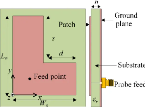
A LPA consists of a patch having WoxLo outer conductor with dxs

slot size as shown in Fig. 1. The patch is placed on a ϵr substrate

with h height on a ground conductor. The designed LPA has Lo=30,

Wo=25, s=10, d=8, h=1.57 (mm) and ϵr=2.33. The antenna is feed

at the point of x=2.03 mm and y=2.44 mm. The LPA is modelled and simulated by means of MoM-based Hyper Lynx® 3D EM which is an efficient CEM packed software. The simulated LPA operates at frequency of 3.125 GHz.

Fig. 1.The geometry of designed LPA

3. Equivalent Circuit Model

The proposed approach for EC model is illustrated on the LPA geometry in Fig. 2 and according formed topology is given Fig. 3. Each branch is modeled with four lumped elements.

Fig. 2. EC model representation on the LPA geometry

The patch conductor is represented with a serial resistance (R11) and inductance (L1) pair for taking into accounts its copper loss and magnetic radiation. Similarly, substrate is represented with a parallel resistance (R12) and capacitance (C1) pair for considering the dielectric loss and electric field. Since the two monopole

patches are combined in parallel, the elements related to these branches are connected in parallel. The consequent EC model is depicted in Fig. 3.

Fig. 3.The proposed topology of EC model for the LPA

Equivalent input impedance equation can be easily derived from the EC model. The input impedance Zin is thereciprocal of equivalent input admittance Yin,

𝑍𝑖𝑛=

1

𝑌𝑖𝑛 (1)

The equivalent input admittance is the sum of admittance of Branches 1 and 2, 𝑌𝑖𝑛= 𝑌1+ 𝑌2 (2) where, 𝑌1= 1 𝑍1 (3a) 𝑌2= 1 𝑍2 (3b)

The impedance of each branch is summed as two serial impedances, for Branch 1 and 2,

𝑍1= 𝑍11+ 𝑍12 (4a)

𝑍2= 𝑍21+ 𝑍22 (4b)

here,

𝑍11= 𝑅11+ 𝑗𝜔𝐿1 (5a)

𝑍21= 𝑅21+ 𝑗𝜔𝐿2 (5a)

andZ12 and Z22 are the impedances of parallel sub-branches including capacitances, 𝑍12= 1 𝑌12 (6a) 𝑍22= 1 𝑌22 (6b) where,Y12 and Y22 are the admittances of the parallel sub-branches,

𝑌12= 1 𝑅12+ 𝑗𝜔𝐶1 (7a) 𝑌22= 1 𝑅22+ 𝑗𝜔𝐶2 (7b) Finally, the equivalent input impedance Zin can be calculated by substituting (2)-(7) into (1). The input impedance can be also written in complex form as,

𝑍𝑖𝑛= 𝑅𝑖𝑛+ 𝑗𝑋𝑖𝑛 (8)

The following equation determined from (8) expresses the reflection coefficient Γ,

Γ=𝑍𝑖𝑛−𝑍𝑜

𝑍𝑖𝑛+𝑍𝑜 (9)

and thus the complex reflection coefficient can be calculated by taking the reference input impedance of Zo = 50 Ω, and therefore the complex reflection coefficient will be,

Γ=𝑍𝑖𝑛−50

𝑍𝑖𝑛+50 (10)

Consequently, return loss (-|S11|) of LPA can be calculated from (10) as follows

𝑅𝑒𝑡𝑢𝑟𝑛 𝐿𝑜𝑠𝑠 (𝑅𝐿) = −20𝑙𝑜𝑔|Γ| (11)

4. Procedures for Constructing the Equivalent

Circuit Elements

4.1. Definition

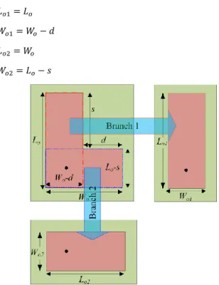
It is assumed that the LPA behaves like two monopole patch radiators. Therefore, the LPA can be represented by two monopole branches as shown in Fig. 4. Branch 1 and 2 respectively stand for long and short monopoles. Their dimensions can be redefined as,

𝐿𝑜1= 𝐿𝑜 (12a)

𝑊𝑜1= 𝑊𝑜− 𝑑 (12b)

𝐿𝑜2= 𝑊𝑜 (12c)

𝑊𝑜2= 𝐿𝑜− 𝑠 (12d)

Fig. 4. Branch representation of the LPA geometry

It is evident that the field radiating at the edges of the monopoles propagates in the substrate and the air. An effective dielectric constant should be regarded and it will be inherently between the dielectric constants of the substrate and the air. Effective dielectric

constant ϵreff in (13)is considered to approximate the dielectric

constant of the substrate to the air [25].

𝜖𝑟𝑒𝑓𝑓=𝜖𝑟₂+1+𝜖𝑟₂−1[1 + 10_𝑊ℎ

𝑜]

−1 2⁄

(13) Likewise, monopole patch lengths look electrically longer than the real length, and therefore an edge extension should be regarded for patch length. The effective lengths expressions taking into account the edge extensions are given as follow,

𝐿𝑜1𝑒𝑓𝑓= 𝐿𝑜1+ ∆𝐿𝑜1 (14a)

𝐿𝑜2𝑒𝑓𝑓= 𝐿𝑜2+ ∆𝐿𝑜2 (14b) where, the length extensions of ΔLo1 and ΔLo2 are treated as optimization variables, and they will be found by optimization. In constructing the EC elements, it is inspired from the lumped element definition of MTL[23]. Similarly, the following expressions (15) including effective lengths and substrate properties are formed in order to construct the effective EC elements containing the antenna’s physical and electrical properties. 𝐶1= ∆𝐶1𝐿𝑜1𝑒𝑓𝑓(𝑊𝑜1 ℎ ) 𝜖𝑟𝑒𝑓𝑓𝜖𝑜 (15a) 𝐶2= ∆𝐶2𝐿𝑜2𝑒𝑓𝑓( 𝑊𝑜2 ℎ ) 𝜖𝑟𝑒𝑓𝑓𝜖𝑜 (15b) 𝐿1= ∆𝐿1𝐿𝑜1𝑒𝑓𝑓( ℎ 𝑊𝑜1) 𝜇𝑜 (15c) 𝐿2= ∆𝐿2𝐿𝑜2𝑒𝑓𝑓( ℎ 𝑊𝑜2) 𝜇𝑜 (15d) 𝑅11= ∆𝑅11𝐿𝑜1𝑒𝑓𝑓(𝐿𝑜1 𝑊𝑜1) (15e) 𝑅12= ∆𝑅12𝐿𝑜1𝑒𝑓𝑓(_𝑊ℎ 𝑜1) (15f) 𝑅21= ∆𝑅21𝐿𝑜2𝑒𝑓𝑓( 𝐿𝑜2 𝑊𝑜2) (15g) 𝑅22= ∆𝑅22𝐿𝑜2𝑒𝑓𝑓( ℎ 𝑊𝑜2) (15h)

where, ϵo and µo permittivity and permeability of free space,

respectively. ΔC1, ΔC2, ΔL1, ΔL2, ΔR11, ΔR12, ΔR21 and ΔR22 which will be determined by optimization are inserted to the EC element expressions to represent the changes in the elements due to the operating as radiators rather than MTLs.

4.2. Optimization

The EC element’s expressions in (15) are optimized using DE since it is a reliable and versatile optimizer based on population, and it has gained popularity in electromagnetic applications in which the number of variables tends to be higher.

The expressionsare optimized to minimize the objective function of RMSE, 𝑅𝑀𝑆𝐸 = √∑ (𝑅𝐿𝑐𝑎𝑙𝑖 −𝑅𝐿𝑠𝑖𝑚𝑖 ) 2 𝑓𝑛 𝑖=1 𝑓𝑛 (16)

where, RLi _{is the return loss value at frequency index of i varies}

between 2 and 4 GHz on 161 discrete frequency points offn.

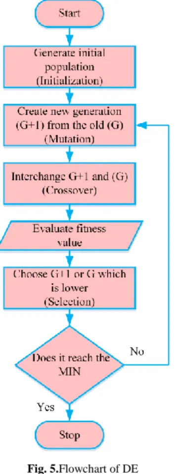
Subscriptionscal and simrespectively denote the calculation by the EC model in (11) and the simulation by HyperLynx® 3D EM. The set parameters of DE optimization are population size: 30, mutation rate: 0.85, crossover rate: 0.7, maximum iteration number: 5000. The upper and lower limits of the optimization variables are given in Table 1.As outlined in Fig. 5, DE performs the optimization by four operators: Initialization, mutation, crossover and selection. For briefly expaining the working mechanism of the DE, the first iteration is hereby addressed: In initial phase, the DE randomly creates a new generation (G=0) for searching population including chromosomes composed of genes within upper and lower limits. Each gene corresponds to optimization variable. The objective values for each initial gene are evaluated by substituting the initial generation into the objective function. In mutation phase, the DE then mutates all chromosomes

for producing a new generation (G+1)from the old genes (initial genes for first generation) as amount allowed by mutation rate. In crossover phase, new genes survive if a random value (0-1) is less than the crossover rate. Finally, chromosomes which have lower objective value either new or old generations are chosen in selection phase. Thus the same iterations will be continued until the maximum iteration number(MIN).

Fig. 5.Flowchart of DE Table 1. Upper and lower limits of optimization variables

# Optimization

Variables Lower limit Upper limit

1 ΔLo1 0 2 2 ΔLo2 0 2 3 ΔC1 0 100 4 ΔC2 0 100 5 ΔL1 0 100 6 ΔL2 0 100 7 ΔR11 0 100 8 ΔR12 0 108 9 ΔR21 0 100 10 ΔR22 0 108

5. Results and Comparison

After the optimization is accomplished, the final values of optimization variables are achieved as given in Table 2. The DE finds the variables with RMSE of 0.025.It should be noted that different EC models with more branches and elements, and also with different topology are essayed for the LPA, as well. Satisfactory results are obtained with only the proposed EC model in Fig. 3. The expressions in (17)belonging to the EC elements are achieved by substituting the values in Table 2 into (15).

Table 2. Optimization variables of EC model found by the DE

# Optimization Variable Value 1 ΔLo1 1.2945 2 ΔLo2 0.1639 3 ΔC1 9.1531 4 ΔC2 0.0031 5 ΔL1 0.6665 6 ΔL2 0.4991 7 ΔR11 17.2182 8 ΔR12 1.0x108 9 ΔR21 39.6090 10 ΔR22 3754375.42 𝐶1= 9.1531 ∙ 1.3245 (_0.001570.017) 2.1862 ∙ 8.854 ∙ 10−12 _(17a) 𝐶2= 0.0031 ∙ 0.1889 ( 0.02 0.00157) 2.1862 ∙ 8.854 ∙ 10 −12 _(17b) 𝐿1= 0.6665 ∙ 1.3245 ( 0.00157 0.017 ) 1.256 ∙ 10 −6 _(17c) 𝐿2= 0.4991 ∙ 0.1889 ( 0.00157 0.02 ) 1.256 ∙ 10 −6 _(17d) 𝑅11= 17.2182 ∙ 1.3245 (0.03 0.017) (17e) 𝑅12= 1.0x108∙ 1.3245 ( 0.00157 0.017 ) (17f) 𝑅21= 39.6090 ∙ 0.1889 ( 0.025 0.02) (17g) 𝑅22= 3754375.42 ∙ 0.1889 (0.00157_0.02 ) (17h)

Optimal EC element values calculated by (17) are achieved in Table 3

Table 3.Optimal EC element values by the DE

# EC Element Value 1 C1 0.02537 pF 2 C2 0.1459 pF 3 L1 102.45 nH 4 L2 9.301 nH 5 R11 40.246 Ω 6 R12 12.232 MΩ 7 R21 9.3537 Ω 8 R22 55.678 KΩ

The calculated and simulated return loss plots of the EC modelare comparatively presented in Fig. 6. In order to validate the EC model, the return loss is further compared with the measurement result of the LPA in [24]. From the figure, the calculated plot is agree well with both simulated and measured ones. Especially, the calculated return loss almost the same as the simulated results. Calculated resonant frequency of3.125 GHz respectively confirms the simulated and measured resonant frequencies of 3.125 GHz and 3.13 GHz. The simulated and calculated bandwidths are very close to each other and it is about 100 MHz. The quality factor is

𝑄 = 𝑓𝑟

𝐵𝑊 (18)

where, fr is the resonant frequency and BW is the bandwidth of the

Fig. 6. Return loss plots of simulated, calculated and measured [21] LPA

The equivalent input impedance is defined in (8) is plotted as real and imaginary parts, Rin and Xin, respectively in Fig. 7. Maximum Rin occurs 397.85 Ω at 3.25 GHz, while maximum and minimum Xin respectively takes place -5.28 Ω at 3.125 GHz and -302.14 Ω at 3.275 GHz.

Fig. 7. Calculated input impedance of the LPA

6. Conclusion

In this study, a novel EC model with eight lumped elements is proposed for the LPA. The EC model consists of two parallel branches each has two serial impedance of a serial inductance and resistance pair and a parallel capacitance resistance pair. The eight lumped element expression are formed by inspiring from element definition of MTL, hence the element expressions cover the antenna’s physical and electrical parameters accompanying with optimization variables. The optimization variables represent the changing in antenna dimension and lumped element values due to operating as radiator rather than MTL. Return loss equation is derived from the EC model. The DE matches the calculated return loss to the simulated to minimize the objective function of RMSE between those return loss results. The lumped elements of EC model are optimally found with RMSE of 0.025. Therefore, the designed EC model is corroborated through the simulated and measured LPA. The return loss of EC model well fits to the simulated and measured results. Finally, the complex input impedance of EC model is successfully calculated.

Acknowledgements

The author is thankful to Mustafa Tekbas for valuable helpin this study.

References

[1] W.F. Richards, Y.T. Lo and D.D. Harrisson, “An improved theory for microstrip antennas and applications,”IEEE T. Antenn. Propag.,vol. 29, no. 1, pp. 38-46, 1981.doi: 10.1109/TAP.1981.1142524 [2] A. K. Bhattacharyya and R. Garg, "Generalised transmission line

model for microstrip patches," IEE Proc-H., vol. 132, no. 2, pp. 93-98, 1985.doi: 10.1049/ip-h-2:19850019

[3] A.Toktas, M. B. Bicer, A. Akdagli and A. Kayabasi, “Simple formulas for calculating resonant frequencies of C and Hshaped compact microstrip antennas obtained by using artificial bee colony algorithm,”

J. Electromagn. Waves. App., vol. 25, no. 11-12, pp. 1718-1729, 2011.

doi: 10.1163/156939311797164855

[4] F. Yang, X.-X. Zhang, X. Ye and Y. Rahmat-Samii, "Wide-band E-shaped patch antennas for wireless communications," IEEE T. Antenn.

Propag., vol. 49, no. 7, pp. 1094-1100, 2001.doi: 10.1109/8.933489

[5] Z.N. Chen, “Radiation pattern of a probe fed L-shaped plate antenna,”Microw. Opt. Techn. Lett.,vol. 27, no.6, pp. 410-413, 2000. doi: 10.1002/1098-2760(20001220)27:6<410::AID-MOP13>3.0.CO;2-Y

[6] A.A. Deshmukh and G. Kumar, “Formulation of resonant frequency for compact rectangular microstrip antennas,” Microw. Opt. Techn.

Lett.,vol. 49, no. 2, pp. 498-501, 2007. doi: 10.1002/mop.22161

[7] A. Toktas, M.B. Bicer, A. Kayabasi, D. Ustun, A. Akdagli. and K. Kurt, “A novel and simple expression to accurately calculate the resonant frequency of annular-ring microstrip antennas,” International

Journal of Microwave and Wireless Technologies, vo. 7, no. 6, pp.

727– 733, 2015. doi: 10.1017/S1759078714000890

[8] D. B. Davidson,“Computational electromagnetics for RF and microwave engineering,” Cambridge University Press, Cambridge, United Kingdom, 2005.

[9] A. Taflove, “Computational electrodynamics: The finite-difference time domain method,”Artech House, Boston, 1995.

[10] R.F. Harrington, “Field computation by moment methods,” IEEE Press, Piscataway, N.J., 1993.

[11] E. Oñate, “Structural analysis with the finite element method. Linear Statics,” vol. 1 Basis and Solids,Springer, 2009.

[12] K. C. Gupta, R. Garg, I. J. Bahl, and P. Bhartia, “MicrostripLines and Slotlines,” 2nd Edition, Artech House, Boston, London, 1996. [13] R.Garg, P. Bhartia, I. Bahl,and A. Ittipiboon. “Microstrip antenna

design handbook,”Artech House, Boston, London, 2003.

[14] A. Singh, M. Aneesh, K. Kamakshi, A. Mishra, J. A. Ansari, “Analysis of F-shape microstrip line fed dualband antenna for WLAN applications,”Wirel.Netw.,vol. 20, no. 1, pp. 133-140, 2014. [15] M. Ansarizadeh, A. Ghorbani, and R. A. Abd-Alhameed, "An

approach to equivalent circuit modeling of rectangular microstrip antennas," Prog. Electromagn. Res. B, vol. 8, pp. 77-86, 2008. [16] A. Akdagli andA. Kayabasi, “An accurate computation method based

on artificial neural networks with different learning algorithms for resonant frequency of annular ring microstrip antennas,” Journal of

Computational Electronics, vol.13, no: 4, pp. 1014- 1019, 2014. doi:

10.1007/s10825-014-0624-6

[17] A. Kayabasiand A. Akdagli, “Predicting the resonant frequency of e-shaped compact microstrip antennas by using ANFIS and SVM,” Wireless Personal Communications, vol. 82, no: 3, pp. 1893-1906, 2015, doi: 10.1007/s11277-015- 2321-6.

[18] A. Kayabasi and A. Akdagli, “Usage of ANN and ANFIS methods for computing resonant frequency of slot-loaded compact microstrip antennas,”Journal of the Faculty of Engineering and Architecture of

Gazi University, vol.31, no: 1, pp. 105-117, 2016, Doi:

10.17341/gummfd.71495.

[19] K. Storn and K. Price, Differential evolution - A simple and efficient heuristic for global optimization over continuous spaces, J. Global

Optim., vol. 11, no. 4, pp. 341–359, 1997. doi:10.1023/A:1008202821328

[20] P. Rocca, G. Oliveri and A. Massa, “Differential evolution as applied to electromagnetics,” IEEE Antenn. Propag. Mag.,vol. 53, no. 1,pp. 38–49,2011.

[21] G. R. DeJean and M. M. Tentzeris, "The application of lumped element equivalent circuits approach to the design of single-port microstrip antennas," IEEE T. Antenn. Propag., vol. 55, no. 9, pp. 2468-2472, 2007. doi: 10.1109/TAP.2007.904129

[22] Y.Jawad , J.Hojin , K. Kwanghoand N.Wansoo , “Design, analysis, and equivalent circuit modeling of dual band PIFA using a stub for performance enhancement”, J. Electromagn. Eng. Sci., vol. 3, no. 3, pp. 169-181, 2016.doi: 10.5515/JKIEES.2016.16.3.169

[23] F. T. Ulaby, “Fundamentals of applied electromagnetics,” Prentice-Hall, Inc. Upper Saddle River, NJ, USA, 1997

[24] A. Kayabasi, A. Toktas, A. Akdagli, M. B. Bicer, and D. Ustun, Applications of ANN and ANFIS to predict the resonant frequency of L-shaped compact microstrip antennas,The Applied Computational

Electromagnetics Society (ACES), vo. 29, no. 6 , pp. 460-468, 2014.

[25] M.V. Schneider, “Microstriplines for microwave integrated circuits,”Bell Syst. Tech. J., vol. 48, no. 5, pp. 1421-144, 1969.doi: 10.1002/j.1538-7305.1969.tb04274.x