Structural Determinants of Household Savings in Turkey : 2003-2008

Structural Determinants of Household Savings in Turkey: 2003-2008

BETAM WORKING PAPER SERIES #007

MAY 2012

Structural Determinants of Household Savings in Turkey: 2003-2008

∗

Arda Aktas, Duygu Guner, Seyfettin Gursel

and Gokce Uysal

∗∗

Abstract

Widening current account deficits coupled with low private saving rates in Turkey have started a recent policy debate on how household savings can be increased. Using Household Budget Surveys from 2003 to 2008, we study the structural determinants of household savings in Turkey. We consider various different definitions for savings, including durable consumption goods, education and health. Our findings are robust across different definitions. The results indicate that dependency ratios of households are important determinants of savings. Lower shares of dependent children or dependent elderly in the household imply higher saving rates. Moreover, female labor force participation has significant effects, i.e. households with higher shares of working females, have higher saving rates as well. We also find that households in which the head is self-employed or an employer have higher saving rates. Moreover, households with where pension payments constitute a larger share of income save less. Note that pension payments are always coupled with free health benefits. These findings point to strong evidence of precautionary savings.

Prepared for the World Bank First draft: March, 2010

This draft: June, 2010

∗ _{We would like to thank Onur Altindag, Evren Ceritoglu, Kamer Karakurum-Ozdemir, Ozlem Sarica, Enver Tasti,}

1. Introduction

The positive correlation between investment and economic growth has been well established in the growth literature. Regardless of the direction of the causality, the financing of investment for achieving sustainable rates of economic growth becomes a major concern. For some countries, domestic savings are large enough to accommodate the demand for funds, whereas in others, such as Turkey, domestic savings are less than adequate. In this case, investments are financed by foreign savings, causing large current account deficits which make economic growth unsustainable in the long run. Therefore, there are increased efforts to stimulate domestic savings to weaken the dependency on foreign funds.

Especially in developing countries, the determinants of saving rates are examined empirically from the macroeconomic perspective due to lack of adequate data. Using time series data, the effects of various macroeconomic and demographic variables1 on savings are examined, however many of them have statistically insignificant effects and/or the estimated effects are not consistent with the theory. In short, the vast empirical literature of savings using macro data provides ambiguous results.

Savings are done by the government, firms and households. Focusing on aggregated data does not provide any insight on the determinants of savings at the household level, making it difficult to develop policies to stimulate household savings. Furthermore, using aggregate data ignores the heterogeneity in socioeconomic and demographic characteristics across households. Consequently, there is a vast literature on the determinants of savings using household level data.

The most common motives for household savings in the literature can be grouped into the following categories: to finance expected life time expenditures (such as house or apartment purchases); to finance unexpected losses of income (precautionary savings); to provide resources for retirement and bequests; to smooth consumption over time and across different states of the world.

Savings are usually measured residually, i.e. as the difference between current income and current consumption. Note that current income may be subject to temporary shocks that may change the saving behavior of the household temporarily, biasing the saving rates. Using household level data with a panel structure enables the identification of temporary income shocks, both aggregate and idiosyncratic. In other words, lack of panel data does not allow for the study of the saving behavior dynamics which may be crucial in understanding the determinants of household savings.

Unfortunately there was no micro level data with a panel structure at the time this paper was written.2

In this paper, we use repeated cross sectional data from the Household Budget Surveys covering the period of 2003 to 2008, to study the determinants of savings at the individual level. We consider several different definitions of savings. Alternative definitions of savings include expenditure on durables, human capital investments such as education and health expenditures and insurance payments.

We find that the implications of the life cycle hypothesis do not hold, savings increase with age for households in which the heads are older than 50. However, this result should be treated with caution given that the cross sectional data may hide substantial cohort effects. Other important determinants of saving at the household level include education, youth (0-14 and 15-30) and elderly dependency ratios, ratio of working women in the household, income and wealth.

We find evidence of precautionary savings in the regression analysis. These findings do not have clear policy implications. Nevertheless, we also find that female labor force participation has a sizeable and positive effect on the saving rate. Therefore, our results suggest that increasing female labor force participation will lead to increased household savings in the future. This finding supports the need for policy stimulating female labor force participation.

1 _{Such as income (temporary / permanent), level of uncertainty (political instability), rates of return (interest rate, inflation...),} domestic and foreign borrowing constraints, fiscal policy, pension system, demographics (old or young age, urbanization…)

2

TURKSTAT has been collecting panel data as a part of the Survey of Income and Living Conditions. However, the micro data has not yet been shared with the general public.

The rest of the paper is organized as follows. After a review of the related literature in the next section, we provide a brief description of the data set used. In this section, we also discuss the variables that may explain saving behavior. Section 4 presents the methodology. The descriptive statistics in Section 5 are followed by the results of the regression analyses in Section 6. The last section concludes and touches briefly on the policy implications.

2. Literature Survey

Especially in developing countries, the determinants of saving rates are examined empirically from the macroeconomic perspective. However, the empirical literature of savings using macro data provides ambiguous results. This is not a surprising result given that savings are done by the government, the firms and the households, and aggregated data hides heterogeneity among and within these groups. Browning and Lusardi (1996) provides a comprehensive review of the recent household savings literature. Several observations highlighted in this survey are very important for empirically estimating saving functions. The authors argue that there are various motives for saving, which imply a significant heterogeneity across households. The motives for saving that they cite are as follows: the discount factor, demographics, real interest rate, and variation in consumption and liquidity constraints.

Browning and Lusardi (1996) emphasize that while it is easy to identify the savers in many societies, it is not trivial to establish the motivation for savings empirically.

Savings are usually measured residually, i.e. as the difference between current income and current consumption. Note that current income may be subject to temporary shocks that may change the saving behavior of the household temporarily, biasing the saving rates. Using household level data with a panel structure enables the identification of temporary income shocks, both aggregate and idiosyncratic. In other words, lack of panel data does not allow for the study of the saving behavior dynamics which may be crucial in understanding the determinants of household savings.

Below are some papers that study the determinants of household savings in a developing country context. Note that panel data is hard to come by in developing countries, making it difficulty to study savings at the household level. One solution is to create synthetic cohorts and study their behavior over time. In cases where this is not possible, the researchers are restricted to the use of a single cross sectional data.

According to Deaton (1990) and Gersovitz (1988), there are numerous reasons why savings behavior in developing countries differ from the stylized facts (i) The life cycle of households is longer than individual members; (ii) savings decisions are taken by the households, and not by individual members (iii) incomes are lower and are less certain in developing countries; (iv) borrowing is more limited in size and outreach and also more costly; (v) saving to accommodate uncertain income is more common than to smooth intertemporal.

Kulikov, Paabut and Staehr (2007) study how household characteristics affect saving behavior in Estonia by using household budget surveys for 2002-2005. They control for income and income variability, various measures of wealth and proxies for credit access as well as household composition, education and the employment status of the household head and of other members of the household. They use two different saving measures, the saving rate and the log saving rate. They find that higher levels of income lead to higher levels of saving. However, wealth related variables such as home ownership and possession of durable goods such as cars have negative effects, if at all, on savings. The proxies for credit access negatively affect saving rates. Bank deposits, financial assets, access to liquidity, household debt and leasing liabilities lead to lower savings. As for the age effects, their results show that younger and older households have higher saving propensities than the middle-aged. In their model, households with higher education save less. They point out that highly educated households face higher and less volatile income streams and therefore need to save less.

Butelmann and Gallego (2000) conduct a similar study for Chile by using 1988 and 1996-1997 Chilean Household Budget Survey. They find that consumption tracks income, however, once demographic characteristics are controlled for, the life cycle hypothesis holds. Besides the regular saving definition, they use broader definitions of saving such as durable goods purchases and investment in human capital. They exclude pension payments from household income which they treat as transfer payment

age saving profile. They study the effects of age, education, income and financial expenses on household savings. The results show that income and education are important determinants.

Burney and Khan (1992) analyze the household saving behavior in Pakistan, using micro level data for 1984-1985 to understand Pakistan’s relatively low saving rate. They use a couple of different saving definitions. In one definition, expenditures on durables and on education are considered as savings. In another, savings are measured as the difference between financial assets and repayments and borrowing. They estimate separate saving functions for rural and urban households, and control for various socioeconomic characteristics and demographic factors. Specifically, they include age of the household head, its square, educational level of the household head, entrepreneurship, employment status and occupation of the household head and the presence of a secondary earner. They also try to capture the effects of household composition through a variable which measures the ratio of

household members who are inactive in the labor market to household size. Their findings are as follows. The dependency ratio and education levels below secondary school affect household savings adversely. Entrepreneurship has a positive but insignificant effect. Households in which the head is unemployed save less. As for the age effects, the results imply that age of the household head enters the savings function in a concave manner, i.e. savings increase with age at a decreasing rate. This is consistent with life-cycle hypothesis. Another important finding of this paper concerns the rural urban divide. The authors find that even if the income levels of the urban households are higher, the saving rates of the rural households are significantly higher.

For Philippines, Bersales at al. (2006) analyze the Family Income and Expenditure Survey (FIES) for seven non-consecutive years. They conduct a descriptive study using micro data. They observe that there are sizeable regional differences in aggregate savings. They also find that saving increases with income and that the lowest income quintile dissaves.

Harris et al. (2002) experiment with a different outcome variable that measures savings by the household’s perception of how much they save. They use an ordered probit method to study the determinants of household savings. Incorporating Melbourne Institute Household Saving Survey and the Westpac-Melbourne Institute of Consumer Sentiment, they find that the age-saving profiles are hump-shaped. However, once they control for income, young individuals save more than their elderly counterparts. The results show that income and wealth are important factors that shift households from lower saving categories to the higher ones. Their analysis also highlights the presence of children as a cause of lower saving rates.

Székely, and Attanasio (2000) study the saving behavior of households in developing countries in Latin America and East Asia. They do not find evidence for the standard life-cycle hypothesis, which implies negative or at least declining saving rates for elderly households, although they suggest that this could reflect institutional differences in pension systems. Authors find a positive relationship between saving and education for all countries. Lower fertility and extended families are other characteristics of East Asia which lead to its comparatively high saving rates.

In order to identify the specific effects of demographic characteristics on Chinese household saving rates, Chamon and Prasad (2008) conduct an analysis which allows them to decompose age, cohort and time effects. After discarding time and cohort effects, authors investigate the relationship between demographics and dramatic increase in saving rates in the 1992-2005 period. They divide this time span in three sub-periods (namely for 1992-1996, 1997-2001 and 2002-2005) and control for (i) demographics of the household: age of the household head, share of household members aged 0-4, 5-9, 10-14, 15-19, and 60 or above (ii) log of household income, (iii) the education level and industry of employment of both the household head and the spouse, and (iv) income, wealth and consumption patterns represented by employment characteristics, a proxy for health risk and home ownership. They find a positive relationship between income and savings which increases over time. Controlling for education, occupation, industry etc, they argue that the positive relationship between income and savings is driven by the fact that households choose to save the transitory part of the idiosyncratic income shocks. Their results indicate a U-shaped age-savings profile and show that households with a relatively younger or older heads have a higher propensity to save. Parallel to the higher savings of elderly, they also find that savings increase in the presence of health risk. According to their estimates, health risk largely drives the sharp increases in aggregate saving rate in China within the period of interest.

In order to quantify the magnitude of precautionary savings, they control for uncertainty through using state owned enterprise (SOE) employment and find an unexpected positive relationship between having a SOE employee in the household and saving rates. They attribute this higher tendency to save among civil servants to SOE reforms China is going through. Moreover, they estimate a positive effect on homeownership for 1992-1996 and 1997-2001, but this effect is reversed in 2002-2005. Finally, they find that presence of children increases household savings, arguing that the households save for the education expenditures of their children.

There are very few studies on the determinants of private saving in Turkey. Van Rijckeghem and Ucer (2009) conduct a very comprehensive study of the savings in Turkey, using both macro and micro level data. Even though the average inflation-adjusted private saving rate is 17.3 percent of GDP between 1998 and 2004, this statistic hides a major fall in saving rates over time. The aggregate private saving rates decrease from around 25% in 1998 to approximately 10 percent in 2005-2006, followed by a slight increase to 11.4 percent in 2007. After discussing the macro developments of the period which may underlie this decline, they use micro data to examine the fall in 2005 using

econometric methods. The micro data used comes from the Household Budget Surveys (HBS), conducted by TURKSTAT. They run the regressions separately for 2004 and 2005, and compare the results across these two years. For the regression analyses, they restrict the data extensively by excluding households of which’s head is under 25, over 70, a student, involuntarily unemployed, disabled or sick, waiting for work or in seasonal employment, as well as eliminating doubtful observations.

Through using a similar explanatory variable set, van Rijckeghem and Ucer (2009) follow Chamon and Prasad’s (2008) methodology and investigate the effects of household characteristics on saving behavior. The authors argue that the serious misreporting of income in the data renders the income variable unusable, so they instrument income with access to hot water and number of rooms in the house corrected for the household size by the OECD equivalency scale. They also include two additional variables controlling for type of social security coverage and a dummy representing those households with an interest income.

According to their results, the most important determinant of household savings is the household income in the first place. Unexpectedly, authors find a negative relationship between education and saving. The authors argue that this is mostly due to greater access to credit for more educated groups. Their analysis does not find consistent effects of homeownership and interest income.

The results also indicate that the age of the household head has no significant effect on saving, but household composition is an important determinant. They find a significant negative effect of

household size, while youth and elderly dependency ratios decrease saving rates. The authors use a proxy for large expected health expenditures, which has a positive, large and statistically significant impact on saving. They also find a small positive effect of the share of housewives in 2004.

As for the variables regarding the employment status of the household head, social security coverage and being self-employed have consistent positive impacts on saving, which the authors attribute to greater exposure to uncertainty. In 2005, they find a positive effect for civil servants.

Using the same data source, HBS of 2002-2006, Cilasun and Kirdar (2009) investigate the age profiles of income, consumption and hence savings of Turkish households within the life-cycle theory

framework. They find that both income and consumption reflects a hump-shape for different age groups, where the latter is flatter then the former. Inconsistent with the life-cycle hypothesis, they highlight that saving rates slightly increase with age. In order to eliminate the effects of temporary income shocks, they use education as a proxy for permanent income and contrary to van Rijckeghem and Ucer (2009), they find that saving increases with education once controlled for age. However, Cilasun and Kirdar (2009) do not employ an econometric model but conduct a very detailed descriptive study.

Ceritoglu (2009) analyzes the effect of labor income risk on household saving decisions in Turkey by using HBS 2003 and 2004. The labor income risk is associated with future labor income uncertainty which is especially important for the working individuals. Hence, this type of uncertainty is expected to

precautionary savings. Besides the traditional saving definition, broader saving definitions that include expenditure on durable goods as saving are used in the analysis.

The econometric results from the pooled OLS regression of household savings shows that having social security and health insurance coverage has negative impact on household savings, while permanent income, real estate ownership, labor income risk and the presence of multiple income earners have significant and positive effects on household savings. Moreover dummy variables for children and family characteristic are found to be statistically insignificant. Two different estimation methods, pooled OLS and pooled tobit models, are employed in the econometric analysis and the econometric results from the pooled tobit regression are similar to the econometric results from pooled OLS regression.

Yilmazer (2010) uses a smaller data set, Survey of Consumer Finances, to study the profile and determinants of household savings in Turkey. The data set used includes information on the distributions of assets and liabilities of households. She finds that savings increase with household income, education and age of the household head. The results also indicate that households with heads who are working, who are self-employed and who are civil servants save more. The data also allows for measuring gold as a saving instrument, 14.8 percent of households have savings in gold. Using HBS of 2002-2005, Yukseler and Turkan (2008) analyze the changing saving pattern among income quintiles and find that first and second income quintiles have a negative saving rate while the higher quintiles’ (4th and 5th) saving rates are above 10 percent. Moreover, they find that saving rates significantly decreased in 2005 mainly due to the sharp increase in household consumption, which they attribute mostly to expanding credit channels.

Ozcan et al. (2003) analyze the determinants of private saving using time series data for the period 1968-1994. Their results indicate that public savings do not crowd out private savings, contrary to previous findings. Also, they find severe borrowing constraints in the economy for the examined period. Their results point to that inflation has positive effects on private savings. Given that the interest rates rose considerably at the beginning of 1990s, they conclude that this may indicate the positive effect of high interest rates on saving during the period under study.

Ozcan et al. (2003) use inflation volatility as a proxy for macroeconomic uncertainty in the economy and find that it has a positive effect on private saving. They argue that the positive relationship between inflation variability and private saving presents an empirical evidence of the precautionary savings. Their empirical analysis is based on time series data, and thus does not provide information about the saving behavior of the households.3 _{However, note that there is evidence of precautionary}

savings at the macro level, and we would expect to find similar results in micro data. 3. The Data

Household saving decisions are usually studied using panel data since the panel structure follows households or individuals over time, enabling the identification of temporary income shocks, both aggregate and idiosyncratic. In the absence of such data, the construction of synthetic cohorts allows disentangling of age, cohort and time effects. Unfortunately, in Turkey, there was no panel data at the time this paper was written, and the period spanned by the repeated cross sections was too short for the construction of synthetic cohorts.

3.1. Household Budget Surveys

The data used in this study are drawn from Household Budget Surveys (HBS) which are conducted annually by the Turkish Statistical Institute (TURKSTAT) since 20034_{. TURKSTAT designed}

3_{Other studies using macro level Turkish data include Yentürk et al. (2009) who examine the interaction among private saving,}

investment and economic growth in Turkey for the period 1987Q1-2003Q1. They find that growth induces savings and investment. Kaya (2009) verifies their results for 1984Q1-2007Q3 by using different model.

4_{Similar surveys were conducted prior to 2002; however, there are coding and data collection discrepancies. Also the data}

available to us were collected in 1994, which was a crisis year with very high levels of inflation. This will cause large discrepancies between the data collected at different months. Since we do not observe the month of participation, it is impossible to correct for possible biases. Given that there are no other surveys of this period which we can use as a point of comparison; we choose not to incorporate the data from 1994 in the current analysis.

Household Budget Surveys as repeated cross sectional surveys that do not have a panel dimension.5 Note that the sample sizes and the questionnaires do not vary much across years with the exception of 2003. In 2003, 25,920 households were interviewed to construct a data set which is representative at the NUTS2 level. However, this was a one-time expansion, and the data sets collected after 2003, contain around 8500 sample households respectively.

HBS survey provides detailed information about family structure, economic conditions, social and demographic characteristics at the individual and household level. It consists of three different data sets, namely, the individual data set, the household data set and the expenditure data set. Individual data set provides information on age, educational attainment, employment status and income levels. Household data set provides information on household items, wealth related variables and living conditions. The expenditure data set, which is collected at the household level, provides detailed information on expenditure items.

Correcting for inflation

Even though all of the expenditure and most of the income items are reported monthly, some income items contain yearly data, such as retirement payments, interest payments, dividends, etc. Therefore, TURKSTAT provides a yearly income variable for all the individuals in the household. This variable is a yearly sum of individual income from all sources. Therefore, when using income and expenditure data, necessary adjustment are made to ensure that the periods of measurement align.

TURKSTAT collects yearly income pertaining to the 12 month period preceding the survey month, and not during the calendar year. In other words, if the household enters the survey on April of 2004, the yearly income refers to the period of 12 months up to April 2004. Due to the fact that households participate in the survey in different months of the year, and that there are considerable regional differences in the inflation rates, TURKSTAT inflates all the income variables to the December of the survey year using an index variable that controls for months as well as regions.6 _{So, in our example,}

the individual income data collected in April 2004 is inflated to December 2004 by an index that also controls for regional differences in inflation. The relevant indices are provided in the individual data sets. This index provided in the individual data sets allows us to inflate the expenditure of the household to the December of the corresponding survey year as well. Hence, the consumption data and the income data are both inflated to the same period and also corrected for regional differences.7 Ceritoglu (2009) deflates household disposable income figures and household consumption

expenditures with annual average consumer price levels for each year. Van Rijckeghem and Ucer (2009) choose to work with the raw data, and do not make any adjustments.

Furthermore, to be able to compare HBS of different years and to conduct analysis with pooled data, we inflate yearly data to December 2008 by using monthly CPI data released by TURKSTAT.

3.2. Variables

Having a choice between using monthly and yearly variables, we choose to work with monthly data given that most of the variables are measured monthly. Therefore, we convert annual income to monthly income by simply dividing by 12. All the other variables are provided on a monthly basis. Saving rates

Conceptually, saving corresponds to a postponement of consumption towards the future, in other words, to a substitution between present and future consumption. Since we have no direct measure of savings in the data, we define it to be the difference between this period’s income and this period’s consumption. In HBS, income corresponds to the household’s total disposable income, excluding

5

The same households are not followed from one month to another or from one year to another. New and different households are interviewed each month to enlarge the coverage of the sample across the country and her regions. The purpose of this design is to reach all geographical regions of the country as well as all income and consumption groups.

6

This information was provided by TURKSTAT through their information services.

7

contributions to mandatory retirement savings and taxes, and including public and private transfers, and pensions, among others. Consumption refers to the sum of all expenditures of the household, including non-durables and durables, goods and services, cash and in-kind, etc.

The only expenditure item that we do not include in consumption is jewelry. Considering the fact that many households keep their savings in the form of gold, especially in areas where banking is not widespread, we believe that gold is widely used as a saving instrument. Unfortunately, there is no data on spending on gold directly. However, one of the expenditure items on the questionnaire collects data on jewelry, clocks and watches. The percentage of households who spend some positive proportion of their income on this item is around 30 percent and quite stable across years, hence we believe that it reflects payments in gold as a form of saving and thus is a component of savings. We do not include expenditure on jewelry in household consumption measures.8

The analysis is extended to include broader definitions of saving such as investment in durable goods purchases and human capital.9 To be exact, we use three different definitions:

The first definition is based on the traditional definition where saving is equal to the difference between income (Y) and consumption (

C

). Therefore the saving rate

S

₁ is determined as the ratio of

unconsumed income to total income.

Y

C

Y

S

1

(

)

−

=

(1)

Second definition of saving (

S

2) treats durable good purchases as another form of saving and

excludes their purchases from the total consumption. Hence the saving rate can be rewritten as Equation (2), where

Dur

_exprepresents the consumption of durable goods.

Y

Dur

C

Y

S

₂

=

(

−

(

−

exp

))

(2)

Finally, in

S

₃ health (

H

_exp) and education (

Edu

_exp) expenditures, which are considered as

investments in human capital and insurance purchases (

Ins

_exp) are considered as saving as well as durable good consumption. The item on insurance in the data set collects data on private insurance payments, and not the mandatory payments made to social security plans.

Y

Edu

H

Ins

Dur

C

Y

S

₃

=

(

−

(

−

exp

−

exp

−

exp

−

exp

))

(3)

A set of alternative definitions of saving rates measure savings as the difference between the logarithm of income and the logarithm of consumption. 10 _{This measure of savings is less affected by}

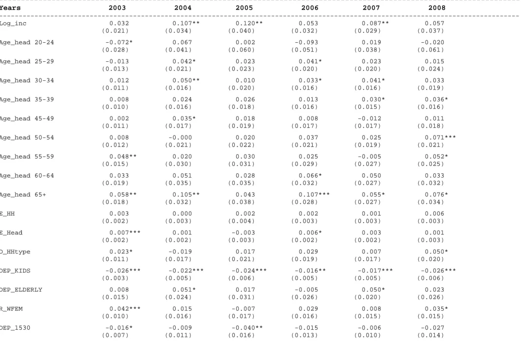
the outliers. We will use it in the regression analyses below. However, we will focus only on the general results of the alternative definitions, reporting the corresponding regression output in the Appendix.

C

Y

S

ln

ln

ln

₁

=

−

)

ln(

ln

ln

S

2

=

Y

−

C

−

Dur

exp

8_{Neither van Rijckeghem and Ucer (2009), nor Ceritoglu (2009) discuss this issue.} 9

This is a usual extension in the literature analyzing household saving. For further information, see Attanasio and Székely (1998) and Gourinchas and Parker (1999), among others.

10 ⎥⎦ ⎤ ⎢⎣ ⎡ + = ⎥⎦ ⎤ ⎢⎣ ⎡ + = ⎥⎦ ⎤ ⎢⎣ ⎡ = C S C S C C Y S ln ln ln1 ln

)

ln(

ln

ln

S

₃

=

Y

−

C

−

Dur

_exp

−

Ins

_exp

−

H

_exp

−

Edu

_exp

Consumption expenditures are calculated as the sum of purchases in the survey month, consumption from the household’s own production, purchases by the household as gifts11_{, and consumption from}

in-kind income and transfers.12

Durable goods are measured as the sum of expenditures on purchases of vehicles, furniture and furnishings, carpets and other floor coverings, household textiles, household appliances, glassware, tableware and household utensils, tools and equipment for house and garden, spare parts for personal transport equipment, telephone equipment, equipment for the reception, recording and reproduction of sound and pictures, photographic and cinematographic equipment and optical instruments, recording media, repair of audio-visual, photographic and information processing equipment, major durables for outdoor recreation, musical instruments and major durables for indoor recreation, equipment for sport, camping and open-air recreation.

Human capital investments include expenditure on education and health. Education expenditures are measured as sum of the pre-primary and primary education, secondary education, post-secondary non-tertiary education and tertiary education as well as individual consumption expenditure of general government on pre-primary and primary education, secondary education, post-secondary non-tertiary education and tertiary education. Health expenditures are measured as the sum of the medical products, appliances and equipment, outpatient services, hospital services. We also include all types of insurance as investment such as life insurance, insurance on the dwelling, health insurance, insurance connected with transport and other insurance.

Household Characteristics

We create some variables to control for household characteristics. The data set provides information on the educational attainment of all household members. Each member is assigned the years of schooling that corresponds to their educational attainment. Then, we average over the years of schooling of all the household members who are older than 15, not enrolled, not sick or disabled. We create a continuous variable,

E

_HH, which measures the average years of schooling of the household member. We also define an education variable for the household head,

E

_head

,

to capture the effect of the years of schooling of household head on saving rate.

As a measure of household composition, three variables are created: dependency ratio for children between the ages of 0 and 14,

DEP

_KIDS, dependency ratio for the elderly, i.e. the individuals in the household over the age of 65 who are not working or looking for work,

DEP

_ELDERLY , and

DEP

₁₅₃₀

,

the ratio of children in the household who are between the ages of 15 and 30, not enrolled in school and are single. In Turkey, most of the young adults live with their parents until they get married, keeping their living costs low and saving for adulthood (wedding, housing, appliances, etc.)13. If so, we expect the saving rate of the household to increase with the ratio of children of ages 15 to 30. On the other hand, a lot of the young adults do not earn enough to be able to live on their own. If this is the case, then they become dependent on their parents as well, which would imply decreased savings for these households.

All of these household composition variables are measured as the ratio of the corresponding group to the number of working members of the household. By including these variables, we measure the impact of having dependents in the household. However, we also would like to take into account the possibility that the elderly in the household may be entitled to retirement benefits and free health care, and thus may contribute to household income. Therefore, we include a variable

R

_PENSION that

measures the ratio of retirement income to total household income.

11_{We include the gifts bought by the households in the consumption regardless of whether the gift was a durable good.} 12

Consumption from income in-kind: Households’ consumption of the goods and services produced or sold in the work place of the household members are treated as consumption from income in-kind. For instance, the allowances of food, clothing etc.

We believe that labor force participation status of the females in the household is an important variable that should be accounted for in the regressions. The labor force status of the women in the household is a major determinant of the bargaining power of the women, who according to recent research save a larger proportion of their income. The variable, denoted by

R

_WFEM

,

measures the ratio of females who work in the household to females who are older than 15, not enrolled, not sick or disabled. Females who work are those who are working for pay, i.e. wage and salary earners, casual workers, entrepreneurs and self-employed women.

Wealth and income variables

HBS lacks data on wealth accumulated in the past. It contains data on household appliances, as well as other household items such as computers, air conditioners, etc. However, the market penetration of these household items changes considerably during the period under study, rendering these variables unusable in the regressions. However, there are some variables correlated with household income and wealth, such as home ownership (

D

_HO), ownership of property other than the one the household resides in14 (

D

_2HO) and car ownership (

D

_CAR). Other variables that convey information on the income and wealth of the household are a dummy for an indoor toilet (

D

_TOI), a dummy for central heating (

D

_HEAT) and the number of rooms per adult equivalent (

R

_ROOM). We also construct a variable,

UNEMP

R

which represents the ratio of unemployed household members to the number of working members in the household.

Furthermore, we expect the entrepreneurship status of the household head to be correlated with wealth accumulation as well as with the income level of the household. In other words, entrepreneurs may save more given that they face higher future uncertainty in income. In addition, owners of small firms may be unable to distinguish the firm’s savings from household savings, causing an upward bias in their saving rates. We create a dummy variable that returns 1 if the household head is an employer or is self-employed (

D

_ENT).

In Turkey, the public sector employment contracts may not be dismissed by the State.15 Given that civil servants face almost a zero probability of job loss in the future; their saving behavior will differ significantly from the employees in the private sector. A dummy denoted as

D

_GOV is created for those whose social security benefits are covered by the pension fund of civil servants, i.e. those who are currently working as a civil servant and those who were retired as civil servants.

Households in which the household head is unemployed are suffering from a negative income shock during the survey month and therefore are expected to save less or even dissave during the period of unemployment. The dummy labeled as

D

_UNEMP is created to capture this negative effect.

Those who work in the informal sector lack social security coverage, and face higher unemployment risk in the absence of severance pay. Moreover, earnings are relatively lower in the informal sector. Those who work in the informal sector generally have low levels of education, low tenure and low level of skills, making this labor market state more permanent than temporary. Therefore, we expect

working informally to be correlated with the income and wealth level of the household as well. To control for informal employment of the household head and also as a proxy for the level of income and wealth,

D

_INF is defined as a dummy.

There is free health care in Turkey for those who are not working, not covered by any social security scheme, and who have less than a threshold level of income. Those who are eligible hold “green cards”, and are entitled to free health care.16 _{The existence of a system of free health care decreases}

14_{This dummy is equal to 1 if the household owns more than 1 apartment or house.} 15_{Excluding fixed term contracts.}

16

Even though the program is means-tested, in 2006, 21% of green card holders had income levels higher than the threshold (Gursel et al, 2009).

the need to save for possible health expenditures of the individual. Therefore, the ownership of a “green card” indicates a low income level, unemployment, inactivity or informal employment, as well as weaker incentives to save. This dummy is denoted as

D

_GC.

We include a dummy variable for household heads who are employed in agriculture (

D

_HAGR), which we believe captures the urban rural divide. Therefore, we do not include a separate dummy for rural areas in the regressions.17

Restricting the sample

When constructing the data used in this paper, we excluded the households where the members are not part of a family, the head is an unpaid family worker18, the head is younger than 20. We also excluded the individuals in the household who were coded as workers for the family or are unrelated. Households in which income and/or spending were negative and in which savings as measured by

S

₂

were in the lowest percentile were dropped. Since these observations are very few, we do not expect major changes in the results.

We also conduct the regression analysis on a more restricted sample where all the household heads are working. This sample allows us to abstract from the households who may be experiencing transitory income shocks (e.g. those where the head is unemployed) and from the households where the head is retired.

4. Methodology

The main objective of this paper is to study the main determinants of household saving behavior. Household savings may differ considerably throughout the life cycle. When using a single cross section, it is impossible to disentangle the age effects, the cohort effects and the year effects.

Therefore, economists use panel data whenever possible and synthetic cohort analysis in its absence. In the synthetic cohort analysis, observations are grouped according to the birth year of the household head. This allows the researcher to follow cohorts through the life cycle while controlling for cohort effect and year effects. However, Turkish data does not allow for the construction of well-measured cohorts, i.e. age data is provided in 5-year groups for 2006-2008. Moreover, our analysis covers the period between 2003 and 2008 which is too short. Therefore, our empirical analysis will be based on a repeated cross section analysis of household saving behavior.

The methodology used is two-fold (i) modeling saving equations and estimating the determinants of savings using two stage least squares estimation for each unique saving definition, (ii) investigating the year effects using a pooled data set where we also control for heteroscedasticity.

As explained above, using log income as an explanatory variable in the savings equation is common practice in the literature. However, given potentially serious measurement error and the endogeneity of household income, we do not directly include income in the estimation analysis, but use instruments to control for its effects on saving rates. Log of income is instrumented with the ratio of unemployed, the dummy for indoor toilet, the dummy for central heating and the number of rooms per adult equivalent. The regression results of the first stage regressions are provided in the Appendix. Note that in the first stage, we include the instruments as well as all the explanatory variables in the savings equation to increase the efficiency of the model.

17

We have experimented with a dummy for rural areas, the coefficient on the rural dummy is not significant when we control for agricultural employment of the household head.

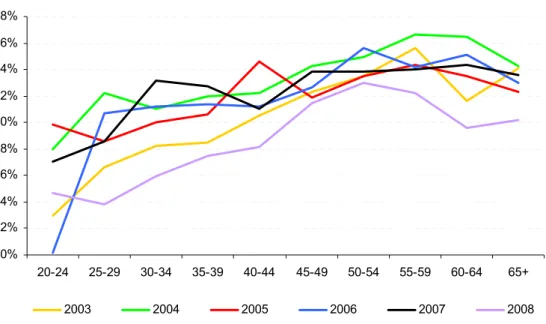
ε

+

+

+

+

+

+

+

+

+

+

+

+

+

+

+

+

+

+

+

=

∑

PENSION GC HAGR UNEMP INF ENT GOV CAR HO HO WFEM ELDERLY KIDS HHtype HH head head

R

D

D

D

D

D

D

D

D

D

R

DEP

DEP

DEP

D

E

E

A

inc

S

2 1530

)

log(

where the first term is the log of income, the subsequent two terms in the right-hand side represents the characteristics of the household head; a dummy set for age (

A

_head) and years of schooling (

E

_head) respectively. Average years of schooling of the household members will be represented by

E

_HH.

HHtype

D

is a dummy variable indicating an extended family. The controls for the household

composition are

DEP

_KIDS,

DEP

_ELDERLY and

DEP

₁₅₃₀represents the dependency ratios of children younger than 14, of elderly and of children between the ages of 15 and 30 respectively.

R

_WFEM demonstrates the ratio of number of working females to household size.

Wealth of the household will be characterized by dummies representing home ownership (

D

_HO), the possession of an additional property (

D

_2HO) and car ownership (

D

_CAR). The model also includes proxies for income such as a dummy for household heads who are employed in public sector (

D

_GOV), a dummy for employer and self-employed household heads (

D

_ENT), a dummy for informally employed household head (

D

_INF) and another dummy for unemployed household heads (

D

_UNEMP). Additional controls are a dummy for green card ownership (

D

_GC), which indicates that the per capita household income is below a certain level and the share of pensions in the total household income (

R

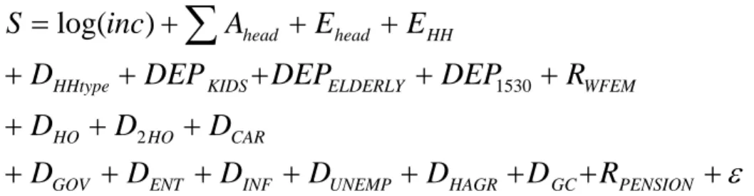
_PENSION). 5. Descriptive Statistics

Table 1 summarizes various measures of savings across different years included in the analyses. When calculating the mean saving rates, we use the income weights of households to aggregate. In the tabulations that follow, we report the median saving rates given that the distribution is skewed and hence the mean saving rates may not reflect the central tendency well. Clearly the median saving rates are more stable across different definitions and years, thus seem to be less influenced by the outliers. Another transformation widely used is the log transformation. The corresponding saving rates are also provided in Table 1. Clearly, using logs also diminishes the effects of outliers.

According to the first definition S1, where saving is the difference between income and consumption,

median savings are the lowest in 2008 at 1.76%, and highest in 2004 at 7.98%. It is easy to see that the variation between years is reasonable if we exclude 2008. Also, note that we find a lower saving rate for 2005 in line with the work of van Rijckeghem and Ucer (2009). They find 17% for 2004 and 10% for 2005. Ceritoglu (2009) finds 17% for a pooled sample of 2003 and 2004.19

The saving rates calculated from household level data in the international context are similar to those found for Turkey. Using somewhat older data sets, Denizer and Wolf (1998) calculates saving rates of 24.8% for Bulgaria, 11.2% for Hungary and 16.5% for Poland. Kulikov et al. (2007) calculate saving rates between 5.6% and 15.1% for Estonia. Chamon and Prasad (2008) calculate saving rates between 14.3% and 22.4% for China from 1990 to 2005.

19 _Van

Rjickeghem and Ucer (2009) do not impose any restrictions on the data at this point. Ceritoglu (2009) restricts his sample to households where the saving rate is higher than -50%.

Table 1 Saving rates 2003-2008 2003 2004 2005 2006 2007 2008 Mean S1 13.71% 13.14% 6.88% 7.97% 9.98% 5.88% S2 20.05% 20.89% 17.90% 18.63% 18.22% 16.73% S3 23.33% 24.66% 22.10% 22.86% 22.36% 20.35% Median S1 7.06% 7.98% 5.27% 6.22% 7.19% 1.76% S2 10.95% 13.47% 11.96% 12.53% 12.79% 9.28% S3 13.84% 16.38% 15.51% 16.12% 15.80% 12.17% Median ln S1 7.32% 8.31% 5.42% 6.43% 7.46% 1.79% ln S2 11.60% 14.47% 12.73% 13.39% 13.69% 9.74% ln S3 14.89% 17.89% 16.85% 17.57% 17.20% 12.96% Number of observations 25293 8380 8387 8397 8372 8336 As expected, the saving rates increase as we widen the scope of savings. When we include

expenditure on durables in savings (S2), we see that the saving rates increase by around 5 percentage

points. Again, we observe a decrease in the saving rates in 2008, though less pronounced. When the human capital expenditures are also included in savings (S3), the median saving rates increase to

12-16 percent.

We see a sizeable drop in the saving rates, both in means and medians, in 2008, especially in S1

where durables, human capital investments and insurance payments are included in household expenditures. Note that the decreases in the saving rates are not as pronounced in the wider saving definitions. This implies that the households have invested in durables and human capital during 2008; however, this is contradicted by the macro level data presented in Table 2 where the total

consumption expenditures, expenditure on durables, and expenditure on durables as a percent of total consumption expenditures are provided. We observe that there is actually a decrease in durable expenditures in 2008. One major difference between the definition of expenditures on durables in the macro data and in our analysis arises from the way the cars are treated. In the aggregate consumption data, new car purchases are included under Transportation; however, we include them as durables in our analysis. We will discuss the decrease in saving rates in 2008 further below.

Table 2 Total Consumption Expenditures and Expenditure on Durables, 1998 prices Consumption Expenditures

Furnishing, Household Equipment and Routine Maintenance of the House

As a % of Total Consumption Expenditures 2003 57,160,510 5,563,577 9.7% 2004 62,966,589 6,468,312 10.3% 2005 67,704,926 7,903,795 11.7% 2006 70,792,710 8,325,526 11.8% 2007 74,106,803 8,558,280 11.5% 2008 73,956,687 7,890,254 10.7% Source: TURKSTAT

In line with the literature, we choose to report our results using S2, which includes expenditures on

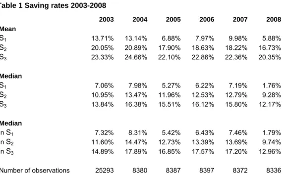
The statistics in Table 3 should be interpreted with caution, and by considering the fact that they are descriptive statistics. 20

Table 3 Median saving rates by certain characteristics

2003 2004 2005 2006 2007 2008

Years

Household composition Age of the head of household

20-24 3.01% 7.95% 9.83% 0.14% 7.08% 4.69% 25-29 6.63% 12.23% 8.54% 10.68% 8.56% 3.85% 30-34 8.20% 11.00% 10.04% 11.18% 13.20% 5.95% 35-39 8.49% 12.01% 10.58% 11.34% 12.75% 7.46% 40-44 10.54% 12.25% 14.62% 11.19% 11.07% 8.19% 45-49 12.34% 14.30% 11.85% 12.65% 13.82% 11.44% 50-54 13.46% 14.92% 13.46% 15.64% 13.84% 13.00% 55-59 15.62% 16.60% 14.33% 14.18% 14.00% 12.26% 60-64 11.59% 16.44% 13.54% 15.11% 14.34% 9.62% 65+ 14.08% 14.24% 12.29% 13.00% 13.58% 10.20%

Years of schooling - head of household

Illiterate or not a graduate 7.44% 8.30% 4.51% 8.38% 8.03% 7.61% Primary school 9.25% 11.95% 10.74% 10.56% 11.69% 6.06% Primary education 9.61% 13.47% 11.48% 10.87% 11.68% 7.33% Secondary education 12.92% 16.09% 15.09% 14.67% 15.53% 10.10% College 17.43% 16.47% 19.37% 20.23% 20.70% 20.36% University 23.09% 23.15% 25.16% 26.47% 23.43% 23.05% Graduate school 26.86% 22.77% 20.15% 19.90% 24.24% 25.65%

Average years of schooling of the household members

Below mean 7.66% 9.37% 5.84% 9.30% 8.76% 5.86% Above mean 11.89% 14.44% 13.92% 13.38% 13.96% 10.15%

Household type

Nuclear family 10.10% 6.47% 11.36% 12.06% 12.14% 7.87% Extended family 15.46% 7.81% 15.39% 14.19% 14.94% 15.23%

Children dependency ratio

Below mean 12.51% 15.23% 13.85% 14.01% 13.71% 11.02% Above mean 7.23% 8.65% 6.32% 7.97% 9.58% 3.08%

Elderly dependency ratio

Below mean 10.29% 13.06% 11.67% 12.30% 12.12% 8.42% Above mean 18.77% 18.37% 16.01% 15.83% 19.37% 19.08%

Young adult dependency ratio

Below the mean 10.56% 13.08% 11.77% 12.36% 12.47% 8.48% Above the mean 12.55% 14.74% 13.27% 13.33% 14.03% 12.12%

Ratio of working females to females

Below mean 9.90% 12.51% 11.17% 11.24% 11.78% 7.85% Above mean 16.44% 17.89% 15.51% 16.64% 16.83% 14.73%

Wealth and Income Home ownership

No 3.80% 8.67% 6.67% 7.72% 8.11% -1.02%

Yes 13.53% 15.09% 14.04% 14.33% 14.42% 13.58%

Own another piece of property

No 9.89% 12.11% 10.64% 11.14% 11.65% 7.50% Yes 20.27% 22.53% 20.61% 20.69% 22.31% 19.68%

Car ownership

No 9.08% 11.28% 9.06% 10.66% 10.98% 6.83% Yes 16.98% 19.39% 19.10% 16.96% 17.30% 15.19%

Household head is an employer or is self-employed

No 7.97% 10.87% 9.44% 10.44% 11.07% 7.53% Yes 20.67% 20.47% 18.49% 18.85% 17.86% 16.16%

Household head works for the government

No 10.23% 12.76% 11.08% 11.77% 11.89% 7.10% Yes 17.48% 20.62% 22.42% 19.65% 24.12% 20.22%

Household head employed in the informal sector

No 11.51% 15.12% 13.96% 13.86% 13.68% 9.88%

Yes 9.48% 8.19% 6.87% 9.21% 10.68% 6.85%

Household head unemployed

No 11.26% 13.65% 12.08% 12.77% 13.04% 9.46%

Yes -1.78% 7.11% 5.28% 2.97% 0.16% 0.64%

At least one member of the household has a green card

No 11.37% 14.26% 14.02% 14.00% 14.27% 10.21%

Yes 1.25% 0.07% -7.99% 0.54% 3.55% 1.00%

Industry the head of household is employed in

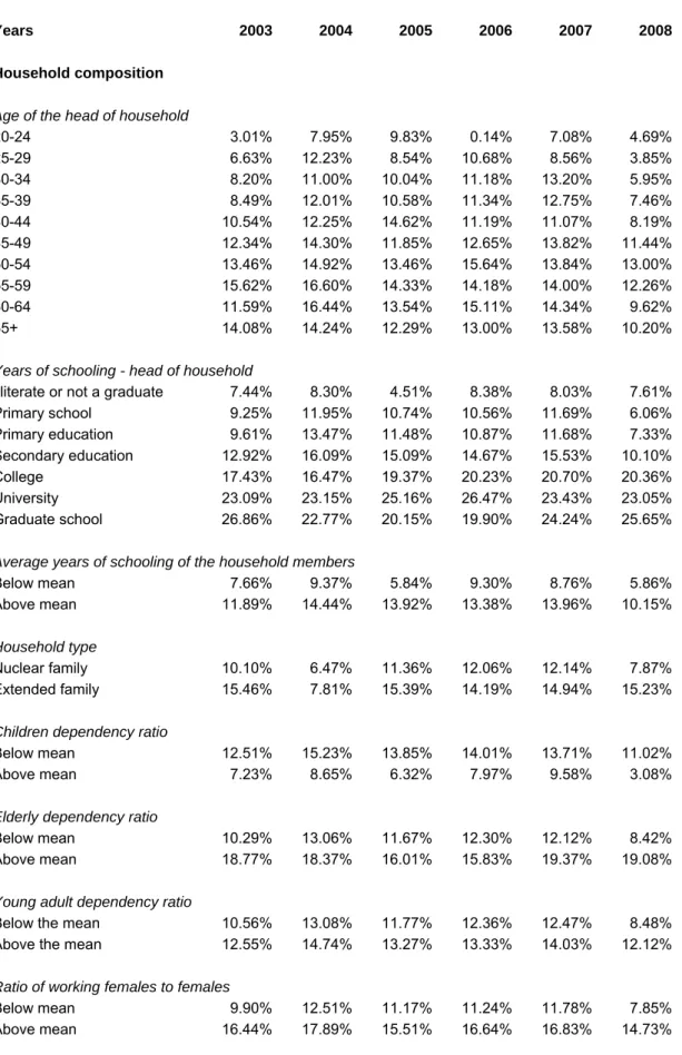
Not working 8.19% 11.58% 8.86% 9.98% 9.92% 7.09% Agriculture 15.99% 9.93% 12.13% 11.14% 12.08% 11.51% Manufacturing and construction 8.17% 11.81% 13.56% 9.67% 10.76% 5.58% Services 13.45% 16.62% 13.98% 16.83% 16.87% 12.25% Income quintiles Lowest -10.34% -8.97% -16.57% -9.97% -5.16% -15.00% 2 3.28% 4.32% 3.87% 7.87% 6.74% -0.75% 3 11.14% 13.69% 12.60% 11.92% 13.17% 6.48% 4 18.09% 19.97% 19.37% 16.05% 17.97% 16.97% Highest 32.10% 33.06% 32.68% 31.23% 28.75% 30.31% First, note that the saving rate increases with the age of the household head. The first age group does not have enough observations to yield significant and stable rates, however, rest of the data points to a stable and increasing relationship between saving rates and age groups of the household head. We even observe a limited decrease in the savings rates for the elderly from 2004 to 2007. The data implies that the age profiles of saving may be hump-shaped. However, studying age saving profiles

from cross sections may cause substantial biases due to cohort effects. Unfortunately, the data sets used in this paper span too short a period of time to allow for the study of cohort effects.

Figure 1 Saving rates by age of head of household

0% 2% 4% 6% 8% 10% 12% 14% 16% 18% 20-24 25-29 30-34 35-39 40-44 45-49 50-54 55-59 60-64 65+ 2003 2004 2005 2006 2007 2008

Lastly, note that the decrease in the saving rates in 2008 varies drastically across different income quintiles. We observe that the households in the higher income quintiles have not lowered their savings at all. However, the lowest three income quintiles experience a major drop in their saving rates. Due to the fact that food consumption constitutes a higher fraction of their expenditures, these groups would have suffered from high inflation rates in food prices in 2007 and 2008. However, we do not observe an increase in the share of food consumption in total income. We also know that the industrial production has started to decline from the 2nd _{quarter on, and that the unemployment rates}

increased drastically in the last quarter in 2008. The data shows that this has disproportionately affected the lowest two income quintiles, where monthly income slightly decreased. On the other hand, the share of housing expenditures and durable good consumption increased drastically in 2008, which may be the underlying reason of decreasing saving rates in 2008. The share of durable good

consumption, which was 7 percent in 2006 and 6 percent in 2007, reached 8 percent in 2008. Similar increases have been observed in rental payments. The share of rental payments in total income, whose average was 20 percent prior to 2008, increased to 25 percent for those in the lowest income quintile. Second and third lowest income quintiles also experienced analogous increases in rental payments in 2008.21

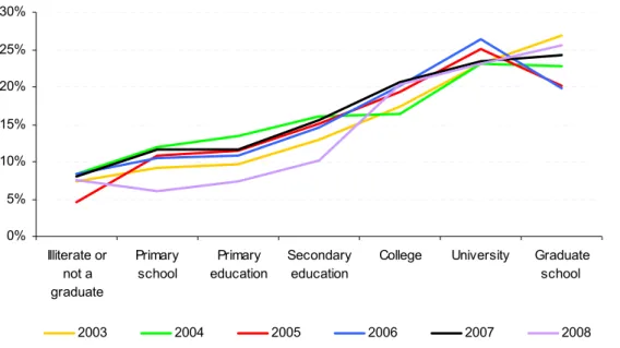
Secondly, we look at the saving rates by educational attainment of the household head and by the average years of schooling of the individuals in the household who are older than 15 years of age and who are not disabled or sick. Note that the educational attainment of the household head is measured in terms of degree completion rather than years of schooling. We assign the minimum years of

schooling required for completion to each individual, and then average over the household to calculate the average years of schooling.

Figure 2 plots the saving rates by the educational level of the household head. Given an education level, the variance of saving rates across different years is much smaller. In other words, education savings profiles are more stable across years than are age savings profiles. The saving rates for a given education level are almost identical across 2005, 2006 and 2007. Note that the saving rates are steadily increasing across education levels. Education levels may be a proxy for income as well as for wealth.

21_{More information is provided in the Appendix.}

We also see that homeownership and savings are positively correlated. Households which are homeowners, also save more. This implies that instead of saving to buy a house, these households see a home or an apartment as a form of saving. Very few households have outstanding debts on their home. If the households were borrowing to buy a house or an apartment, we would have seen it under the related item.

Being a major determinant of income, the employment status of the household head has important implications for savings. Households where the head works for the government, or is self-employed or an employer save more. Contrary to our expectations based on job stability, the data indicates that the households in which the head works in the public sector save more. We believe that there may be selection into the public sector.

Figure 2 Saving rates by education level of the household head

0% 5% 10% 15% 20% 25% 30% Illiterate or not a graduate Primary school Primary education Secondary education

College University Graduate school

2003 2004 2005 2006 2007 2008

Households where the head is unemployed, is employed in the informal sector, or at least one member holds a green card, the saving rates are lower. As for the industry of employment, raw data implies that saving rates in agriculture and in services may be higher. Given that income streams are more random in agriculture, we believe that families employed in agriculture have precautionary savings. On the other hand, higher income levels in the service industry may imply higher saving rates.

6. Regression Analysis

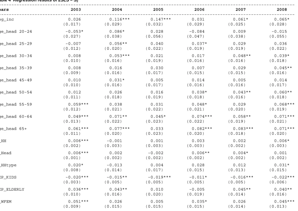
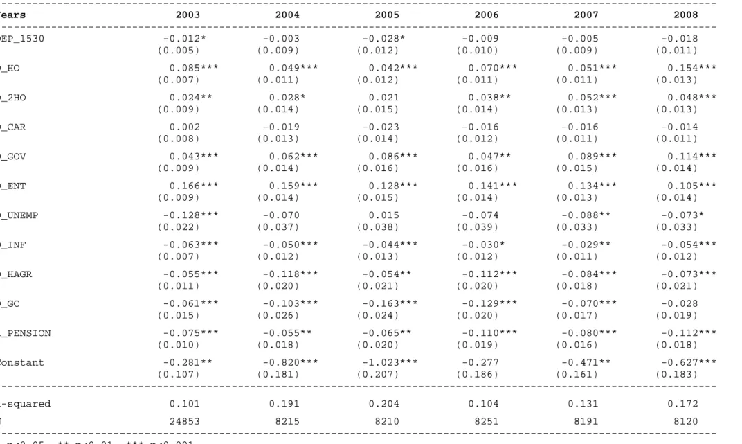
To be able to quantify the marginal effects of a given variable, controlling for all other characteristics, we conduct econometric analyses. We start with a two stage least squares model where all the control variables are included in the model, and log of income is instrumented.22 The first stage results are provided in the Appendix. In Table 4, we report the full sample regression results using S2 which

includes expenditure on durables in the savings. We discuss the results of other definitions and measures briefly, and provide their regression results in the Appendix.23

We find that the households where the head is older save significantly more than the reference category where the household head is 40-44 year olds. The significant coefficients are those that belong to the category of household heads who are more than 50 years old. We observe an increasing age-savings profile in all the years considered. However, the hump-shaped profile in the raw data is not observed here. Note that this result holds even when we control for the number of elderly members as measured by the elderly dependency ratio.

22

We compute Sargan and Basmann tests of overidentifying restrictions for each year and we fail to reject the null to conclude that instruments are exogenous for all years but 2004.

23

The life cycle theory, in its simplest form, predicts that the households run down their assets as they get older. Data do not seem to confirm this prediction. There could be a couple of reasons behind this irregularity. First of all, the elderly may save more and life cycle hypothesis in its simple form may not hold. If this is the case, then we should observe increasing saving rates in Turkey over time due to the compositional effects of the aging population. Secondly, there may be selection bias in households in which the head is older than 65. Only the elderly who have saved and accumulated for retirement can afford to stay as household heads, while the rest move in with their children. In other words, those households who save more can afford to live in their own homes well after their 60s while those who have not saved sufficiently, move in with their children. Therefore, the individuals who remain

household heads above the age of 65 may be those individuals who saved more during their working lives. If this is the case, we would not expect savings to increase as the population ages.

A brief look at the regression results verifies that education has a positive but limited effect on saving rates when we control for income. The education level of the household head and the average education level of the individuals in the household have similar effects on the saving rates. Even though these effects are smaller in comparison to other variables, they are surprisingly consistent across years, both in terms of magnitude and significance. Kirdar and Cilasun (2009) also find a consistently positive relationship between education levels and saving rates.

The coefficient on the dummy for extended family is positive for two years in the sample. Whether a household consists of an extended family is correlated with region and urban / rural divide. Hence, extended families may have restricted access to credit markets, and thus need to save more. Moreover, the household sizes are larger for extended families, implying that they may benefit from economies of scale.

Note that the household composition as measured by the dependency ratio of children 0-14, elderly and children 15-30 in the household affects the saving rates. The presence of children 0-14 in the household implies that the household does not or cannot save as much due to increased

consumption. This is in line with the findings in the literature. On the other hand, if there are more elderly in the household, the saving rates are higher. This is an expected result given that the households expect the health expenditures of the elderly to increase over time. 24 _{However, we must}

also take into account the fact that the elderly with pension plans have a constant stream of income as well as free health care, both of which imply lower savings. We observe that the ratio of pension payments to total household income has significantly negative effects on the saving rates as expected. The coefficient on the dependency ratio of children 15-30 is negative. This is a surprising result given that the young adults reside with their parents and may find it easier to save for the future by

decreasing their living expenses. However, the coefficient is negative, implying that the young adults take this opportunity to increase their consumption. Note that the age of the household head is correlated with the ratio of children 15 to 30 in the household. The potential positive saving effects of young, single and working individuals in the household may be hidden by the higher saving rates of the households with older heads.

The ratio of working females has significant effects on saving rates. The saving rates are increasing in this variable, indicating that the saving behavior of households where more women work is different. These households save more, holding everything else constant. This has important implications for policy in Turkey, especially since there is a lot of room for improvement in Turkey where female labor force participation rates are extremely low.

Note that the coefficient on log of income (as estimated in the first stage by ratio unemployed, dummy for inside toilet, dummy for central heating, room per adult equivalent and all the explanatory variables of the second stage) is significantly positive. In addition, other variables that are correlated with income, but that do not constitute valid instruments for income; also have highly significant and sizeable effects on saving. Remember that we also control for home ownership, car ownership as well as some structural employment indicators of the household head, e.g. entrepreneurship, being a civil servant and working in the informal sector as proxies of income and wealth. We also include variables

24

Rijckeghem and Ucer (2009) find that the saving rates are not affected by the share of elderly in the household, but increase with the health risk of the household.

such as the ownership of a green card, a dummy for the household head being unemployed at the time of the survey and a dummy for the household head working in agriculture.

Car ownership has no significant effects on the savings rate. This result is consistent across years. On the other hand, homeownership and ownership of a second property are positively correlated with saving rates. Since very few of these households have outstanding debt on their homes, we can conclude that in Turkey, households save to buy these items, rather than borrow.25

We find that the households where the head is self-employed or an employer, save more.

Entrepreneurs may face more volatile income streams, which strengthen precautionary motives for saving. This confirms our former intuition.

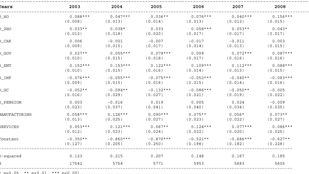
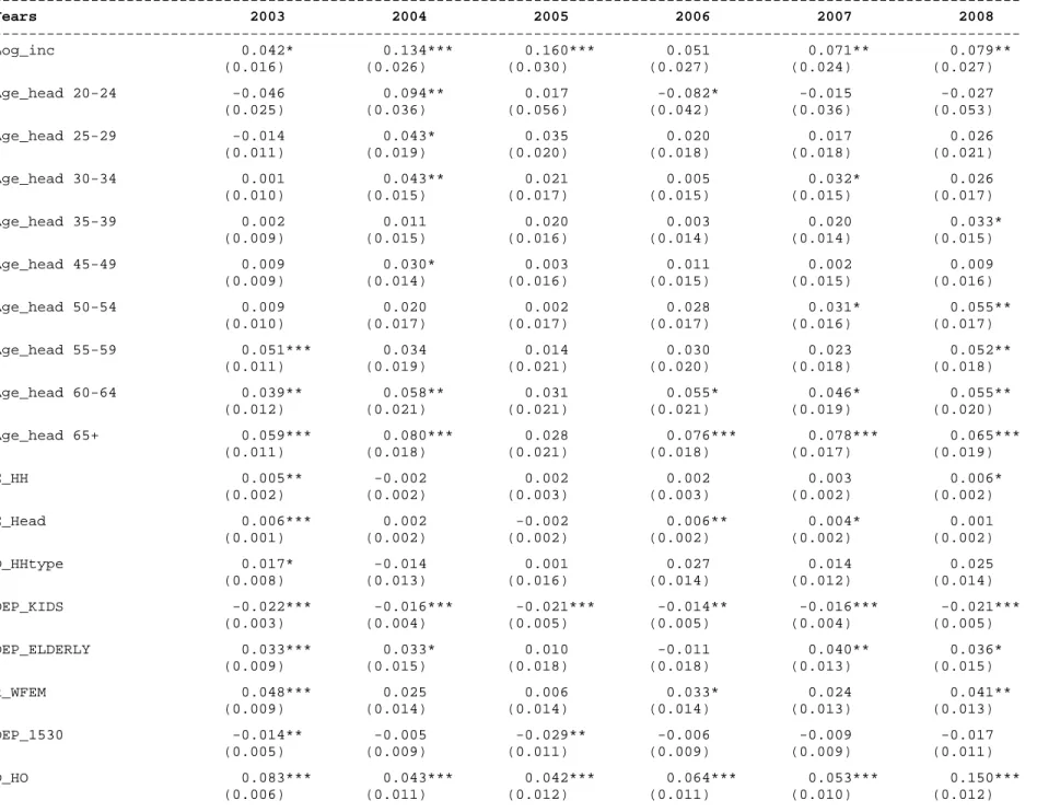
Table 4 Regression results of 2SLS – S2 --- Years 2003 2004 2005 2006 2007 2008 --- Log_inc 0.026 0.116*** 0.147*** 0.031 0.061* 0.065* (0.017) (0.029) (0.032) (0.029) (0.025) (0.028) Age_head 20-24 -0.053* 0.086* 0.028 -0.084 0.009 -0.015 (0.027) (0.038) (0.056) (0.047) (0.038) (0.055) Age_head 25-29 -0.007 0.056** 0.040 0.037* 0.029 0.036 (0.012) (0.020) (0.022) (0.019) (0.019) (0.022) Age_head 30-34 0.008 0.053*** 0.021 0.017 0.048** 0.039* (0.010) (0.016) (0.019) (0.016) (0.016) (0.018) Age_head 35-39 0.008 0.016 0.030 0.007 0.029 0.045** (0.009) (0.016) (0.017) (0.015) (0.015) (0.016) Age_head 45-49 0.010 0.031* 0.005 0.014 0.005 0.014 (0.010) (0.016) (0.017) (0.016) (0.016) (0.017) Age_head 50-54 0.012 0.026 0.016 0.038* 0.043** 0.060** (0.011) (0.018) (0.019) (0.018) (0.016) (0.018) Age_head 55-59 0.059*** 0.038 0.031 0.048* 0.029 0.068*** (0.012) (0.021) (0.022) (0.021) (0.020) (0.019) Age_head 60-64 0.049*** 0.071** 0.045* 0.074*** 0.058** 0.071*** (0.013) (0.022) (0.023) (0.022) (0.019) (0.021) Age_head 65+ 0.061*** 0.077*** 0.033 0.082*** 0.083*** 0.071*** (0.011) (0.020) (0.023) (0.020) (0.018) (0.020) E_HH 0.006*** -0.001 0.001 0.003 0.002 0.006* (0.002) (0.003) (0.003) (0.003) (0.002) (0.003) E_Head 0.006*** 0.002 -0.002 0.006** 0.004* 0.001 (0.001) (0.002) (0.002) (0.002) (0.002) (0.002) D_HHtype 0.020* -0.013 0.004 0.028 0.012 0.031* (0.008) (0.014) (0.017) (0.015) (0.013) (0.015) DEP_KIDS -0.020*** -0.015** -0.019*** -0.011* -0.016*** -0.022*** (0.003) (0.005) (0.005) (0.005) (0.005) (0.006) DEP_ELDERLY 0.036*** 0.043** 0.010 -0.005 0.045** 0.040** (0.010) (0.016) (0.020) (0.019) (0.014) (0.016) R_WFEM 0.051*** 0.026 0.005 0.035* 0.026 0.045*** (0.009) (0.015) (0.015) (0.015) (0.014) (0.013)