Environmental Quality and Energy Import Dynamics: The Tourism
Perspective of the Coastline Mediterranean Countries (CMCs)
Andrew Adewale Alola,[ 1 ] ; Kayode Kolawole Eluwole,[ 2 ] ; Uju Violet Alola,[ 3 ] ; Taiwo Temitope Lasisi,[ 2 ] ; Turgay Avci,[ 2 ]
Abstract
Purpose: The geographical location and the ambiance of the Coastline Mediterranean Countries (CMCs) advantageously present the region as a tourist destination with rich cultures.
Methodology: As such this study investigates the dynamics of energy import and environmental quality in relation to international tourism development for nine coastline Mediterranean countries over the period 1995-2013 using a Pooled Mean Group (PMG) approach.
Findings: While the impacts of energy import, CO2 (here as environmental quality), and GDP on
international tourism receipts are observed to be significant and negative, international tourist arrival expectedly exerts positive and significant impact, all at adjustment speed of 0.19. A heterogeneously robust Granger non-causality test further reveals a strong one-directional causal relationship from energy import to tourism receipts.
Author Information
Reprint Address: Alola, AA (reprint author)
Istanbul Gelisim Univ, Dept Econ & Finance, Istanbul, Turkey. Addresses:
[1 ] Istanbul Gelisim Univ, Dept Econ & Finance, Istanbul, Turkey [ 2 ] Eastern Mediterranean Univ, Gazimagusa, Cyprus
[ 3 ] Istanbul Gelisim Univ, Istanbul, Turkey E-mail Addresses:
[email protected]; [email protected]; [email protected]; [email protected];
Research Implication: The dynamics of the energy market amidst persistent evolution of new source(s) of energy would evidently play a significant role in the region’s tourism sector. It then suggests policy direction to governments of the region and by extension the global tourism market.
Originality: By providing insight into the nexus of environment, energy and tourism development, the current study is the first that addresses the concern in the context of the CMCs.
Keywords: energy import; tourism development; CO2; coastline Mediterranean countries; PMG estimator
1. Introduction
In over six decades, global tourism industry has witnessed increasing and sustained growth which has made the sector an integral component of the world’s economy (Alola & Alola, 2018a; United Nation World Tourism Organization, UNWTO, 2018). The UNWTO (2016) indicates that “Tourism has boasted virtually uninterrupted growth over time, despite occasional shocks, demonstrating the sector’s strength and resilience. International tourist arrivals increased from 25 million globally in 1950 to 278 million in 1980, 674 million in 2000, and 1186 million in 2015”. Also, international tourism receipts have surged from US$2 billion in 1950 to US$1260 billion in 2015 (UNWTO, 2016). The industry has continued to experience hundreds of millions international arrivals in destinations across the globe. These indices significantly placed tourism industry third in world ranking for export and also responsible for ten per cent (10%) of world’s Gross Domestic Product (UNWTO, 2016).
Although tourism has not necessarily been elaborately detailed in the context of energy import, rather handful of energy consumption-tourism nexus have been significantly investigated (Gokmenoglu & Eren, 2019; Zhang & Liu, 2019). But on energy import, Zhao & Wu (2007) noted that growth of industrial production and expansion of transport sectors are core
determinants of China's oil imports. This could account for reason why countries rely on inbound travellers for major economic development which is responsible for the creation of new businesses, international trades, foreign exchange, and many more other indicators. The significant trends observed in tourism industry have attracted the attention of many researchers. Several literatures with empirical evidences have supported the fact that development in tourism will impact economic development positively (Katircioglu, 2009; Kilic & Bayar, 2014; Akadiri, Akadiri & Alola, 2017; Akadiri & Akadiri, 2019). Also, few other studies have varied assertions on the specific economic indicators responsible for the actual economic growth. Some consider foreign exchange (Dritsakis, 2004), tourism-led growth (Al-mulali, Fereidouni, Lee, & Mohammed, 2014; Tang & Abosedra, 2014; Tang & Abosedra, 2016), and international trade (Rauch & Trindade, 2002; Shan & Wilson, 2001). Paramati, Alam and Chen, (2016) argued that tourism’s impact on economy manifest through the improvement in employment opportunities, income levels, tax revenues, and foreign exchange reserves.
Considerable numbers of studies within the framework of tourism and economic growth have covered the lingering concern of climate change vis-à-vis carbon emissions which is in line with the motivation of this study. The study of the relationship between carbon emission, tourism-led growth and economic growth in general is currently still receiving different perspectives (Lee & Brahmasrene, 2013; Katircioglu, Gokmenoglu & Eren, 2018; Saint Akadiri et al., 2019; Balli et al., 2019; Katircioglu, Cizreliogullari & Katircioglu, 2019; Katircioglu, Cizreliogullari & Katircioglu, 2019; Akadiri, Alola & Akadiri, 2019). However, the current study is aimed at hypothesizing that there is causal nexus of energy security and environmental quality with tourism development in the destination of panel of Coastline Mediterranean Countries (CMCs).
As a result, this study is novel in that it is a paradigm shift from the conventional studies that commonly details the effect of tourism on economy and vice-versa. In addition, the current study injects the novelty of investigating and lauding the specifics of the CMCs (a yet to be explored group of countries). However, by employing the common instrument of economic indicators as clearly elaborated above, this study is believed to enhance extant literature through the following approach:
Firstly, it uses a rather more subtle but important element of tourism receipts2 which
proxy for tourism development. Specifically, energy import3 (a constituent of energy
security) as a constituent of import of good and services is investigated with tourism receipt, a tourism indicator carefully studied in Tang (2013).
Secondly, to the best of authors’ knowledge, the study further advances the research on the Coastline Mediterranean Countries (CMCs) by Alola and Alola (2018b) and Alola, Alola & Akadiri (2019) where CMCs was investigated in the framework of renewable energy. In this case, it specifically focuses on the consideration of how the region’s energy import trend and international tourism receipt are inter-linked.
Also contributing to the existing literatures, this study presents a robust second generation panel data empirical models that accounts for the cross-sectional dependence (CD) by Pesaran (2004). This study additionally employs panel data estimation of cointegration by Westerlund (2007) and the pooled mean group (PMG) to investigate short and long-run equilibrium relationship between tourism receipts and energy import. Like in the previous literatures (see. Dumitrescu and Hurlin, 2012), Granger causality test is favoured to perform the directional relationship between these variables.
2 World Development Indicator, WDI, 2019) presents details on international tourism receipts.
3 World Development Indicator, WDI, 2019) presents details on energy import. The details of the information are available at http://data.worldbank.org/data-catalog/world-development-indicators.
The remaining sections of the paper are arranged such that next section (2) briefly discusses energy import, tourism, and its specifics to coastline Mediterranean countries. Data and empirical model used forms the content of section 3. The results of the estimations are discussed in section 4, and section 5 presents the concluding remark with the research implication.
2. Energy security dynamics
Net energy import is an estimated volume of energy use less of production, and that are measured in oil equivalents (World Development Indicator, WDI, 2019). This account for reason to have a paradigm shift from the seemingly conventional discuss on energy consumption to a salient issue of energy import. Of the US$679.1 billion of imported crude oil in 2016, Asian countries are reported to have highest importation of $331.6 billion worth (49.4% of global import), while European countries, North America, Latin America, Africa and the Oceania were reported to have imported 28.6%, 17.7%, 1.9%, 1.3% and 1.2% worth of global crude oil importation (World Development Indicator, WDI, 2019). The concern is that importation of crude oil has been on a declining trend globally such that none of the known major crude oil importing country has had energy import boost since 2012. This could account for why most recently countries began to domesticate sources of their energy consumption, reliant on the importation of energy has been and still a worrisome research venture. Importantly, countries with total reliant on single suppliers for sources of energy and those supplying nations with limited market base for their energy products have both suddenly identify the relative need for energy diversification as it applies to either of both cases. For instance, European commission reported a concise effort aimed at helping energy suppliers’ diversification of the Southern Gas Corridor through infrastructural expansion that could ease supplies from the Central Asia, the
Middle East, Caspian Basin, and the Eastern Mediterranean Basin to different part of Europe (European Commission, 2017).
2.1 The CMCs: Energy Import and Environmental insights
The countries of the coastlines Mediterranean Sea, except for its small islands are bordered by
twenty-one connecting sovereign nations4. The peculiarity of the entire Mediterranean region
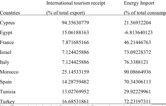
that is naturally endowed with uninterruptedly energy stable region until about two decades ago when energy insecurity rapidly became a growing concern of this touristic hub (Alola & Alola, 2018). Since tourism is also known to be a huge contributor to most of the region’s economic development, it is worth investigating the magnitude of impact between energy import and the tourism sector in the region. The level of unrest in the region, take for instance the devastating and unending Syrian war, economic sanctions against states like Iran and Russia who are the region’s partners, revolution and post-revolution within and around the region and many more factors have largely contributed to energy insecurity of the region (Wilson center, 2015). Now, it could be well-understood why Turkey and Italy which are among the region’s energy import dependents are cooperatively on workable policies that tend to ameliorate energy import challenges (Üstün, 2011). About half of region’s oil and gas needs are currently imported; this unending trend is expected to meet the growing domestic demand. The table 1 below presents the percentage of energy import (except for Egypt that exported more energy) of the investigated countries for the year 2013. Intuitively, more availability of energy is expected to boost economic and social activities across respective countries which are expectedly designed to attract high volume of payments made for all kinds of good and services by the arriving tourists.
4Coastline of the Mediterranean sea is bounded in the northern shore (by Spain, France, Monaco, Italy, Slovenia, Croatia, Bosnia and Herzegovina, Montenegro, Albania, Greece and Turkey), southern shore by Morocco, Algeria, Tunisia, Libya and Egypt), eastern shore (by Syria, Lebanon and Israel) and by the island nations of Cyprus and Malta (Wikipedia).
[Insert Table 1 here].
While studying agricultural land use and tourism impact on renewable energy, Alola and Alola (2018b) notably expressed that tourism activities granger-cause energy consumption. The study informs that investment in tourism results in economic growth and growth in turn results in increased energy consumption. The justification for such association is that tourism growth demands infrastructural developments that will not only claim land meant for sustaining natural ecosystem but will also require energy to power the basic amenities for the infrastructures to be functional. This supports the assertion of Stauvermann and Kumar (2016) which emphasized that economic growth and/or development of tourism islands are a direct function of the impacts of international tourism. As such, Raghoo et al (2015) revealed that the dependent of the Small Island Development States (SIDS) on fossil fuels is the reason the countries are largely characterized by the energy security challenges. Having revealed the six dimension of the peculiarity of energy security dimensions of the SIDS countries, Raghoo et al (2015) equally offered potential policy recommendation for the situation. According to Wang et al (2018), renewable energy consumption is as good as mitigating the effect of carbon emissions and utilized as a remedy for energy insecurity in China. However, the link between energy and environmental quality within different perspectives (including tourism) has been widely covered in the extant literature (Alola, 2019 a & b; Bekun, Alola, Bekun & Sarkodie, 2019; Alola & Sarkodie, 2019; Saint Akadiri, et al., 2019).
3. Data and Estimation Techniques 3.1 Data
The annual data used in this study to primarily investigate possible relationship between tourism development and energy security vis-à-vis energy import among the nine (9) of the twenty-one coastline Mediterranean countries are collected from the World Development Indicators (WDI, 2019) of the World Bank database. These countries; Cyprus, Egypt, France, Israel, Italy, Morocco, Spain, Tunisia, and Turkey were selected because of their similar touristic, energy usage pattern, and availability of data for the same investigated periods of 1995 to 2013 (covering nineteen years). Twelve others countries (Albania, Algeria, Croatia, Bosnia and Herzegovina, Greece, Lebanon, Libya, Malta, Montenegro, Slovenia, Syria) were excluded due to lack of information especially for the experimented nineteen years. The variables employed for the investigation are the international tourism receipts-receipts (it largely measures the tourism development of a country vis-a-vis if a country is a tourist destinations), energy import
measured in metric tons the volume of imported source of energy, CO2 (metric tons of carbon
emission), tourist arrivals (arrivals) is the number (in hundreds of thousands) of tourist visiting a
destination, and the real Gross Domestic Product (gdp) per capita. The variables arrival, CO2,
and gdp were utilized as control variables in this study, as such controls for other unobserved indicators. Using energy import in lieu of energy consumption function (Asafu-Adjaye, 2000; Alola & Alola, 2018b; Gokmenoglu & Eren, 2019), the empirical model for this investigation is give as follows:
receipts = F(energy import, tourist arrival, CO2, gdp)
Then, applying logarithm to the above model, the possibly presence of heteroskedasticity can be minimized such that the model is represented as:
lnReceipti, t = αi,t + β1 lnEimporti,t + β2 lnarrivals,t + β3 lnC02i,t + β4 lnGdpi,t + εi,t (1)
where αi and β1 are respectively constant and parameter coefficients of the estimates for a given i
= 1, 2, …, n and over corresponding periods t, and ε is the error term of the system.
3.2 Panel unit root tests
Importantly, the variables properties such as the order of integration of the variables are firstly investigated using the panel unit root test before applying the cointegration approach. Rather than assuming homogeneity among the panels which could possibly cast a doubt on the estimation results, second generation panel unit roots techniques developed by Pesaran (2005) is employed. Lastly, Granger causality approach will further indicate the one and two-directional prediction nexus among the estimated variables.
3.2.1 Pesaran (2005) unit root test
This second generation test addresses the question of dependence and correlation that are drawbacks of macroeconomic dynamics and hence in all first generation values of the panel unit root. Pesaran (2005) first uses the Cross-Sectional Augmented Dickey-Fuller (CADF) regression which accounts for possible presence of serial correlation to estimate the ith cross-section in the panel. In furtherance of this, Pesaran (2005) proposed the CIPS statistic that is based on average of an estimated individual CADF statistics.
CADF estimation where each variable for specific country i assumes the value of y at time t is represented as:
Δyit = αi + iyi, t-1 + γiЎt-1 + γi ∆Ўi, t-j + ∆ yi, t-j + εit (2)
where ti (N, T) is the t-statistic of the estimate of i of equation (1) above, and also
CIPS = (1/N) (N, T) (3)
given the H0 = Null hypothesis of all series contain a unit root again the alternative hypothesis of
H1 = fail to reject the H0 (there is evidence of unit root all series).
In Table 1, the results of the estimates above are presented.
3.2.2 Fisher-type unit root test
The Fisher-type test performs either ADF or Phillips–Perron unit-root tests on each panel differently before combining the p-values that produces an overall test of evidence or lack of evidence of unit root across the panels. For similar reason specified above, the Augmented Dickey-Fuller option is adopted here especially as T also grows when N become large.
Equivalently, the Fisher-ADF specification for the unit root test with a lag order selection is given as
∆yit = i* yi, t-1 + ∆ yi, t-1 + zit γ + µi t (4)
but where the both the null (Ho) and the alternative (H1) hypotheses are represented as
Ho: i* = 0H1: i* < 0
also, the H0 = Null hypothesis of all series contain a unit root again the alternative hypothesis of
H1 = fail to reject the H0 ( there is evidence of unit root all series). The result of the estimates
from using the above model is displayed in Table 2.
[Insert Table 2 here].
3.2.3 Hadri LM unit root test
The notable weakness of power in testing against alternative of unit root as implemented in the aforementioned tests and others like the Levin, Lin and Chu (2002) and Im, Pesaran and Shin W (2003) among others, has led to more frequent use of Hadri (2000) LM test. Hadri (2000)
employs panel data that test for the null hypothesis of stationarity against the alternative of a unit root across the estimated panels. Unlike the Fisher-ADF, this test is preferred for cases of large T and moderate N or grows in T equivalently resulting in N becoming large so that each series is expressed as:
yit = γit + βit + εit (5)
where γit is an observed random walk which is expressed as:
γi t = ɤi,t-1 + it (6)
so that εit and it iid (independently identical) zero-mean normal errors.
and the H0-null hypothesis (stationarity test) and the alternative H1 are expressed as follows:
H0: λ = σ2,/ σ2,ε = 0 and H1: λ > 0 (7)
In the entire test types mentioned above, each of the understudying variables, tourism receipts
Receipts), energy import (e-import) e.t.c. is assigned as yt in performing the panel unit root tests
to give estimated results of Table 3.
[Insert Table 3 here]
3.3 The Panel cointegration test
A normally distributed four-panel cointegration test statistics, the Ga , Gt , Pa and Pt that is based
on the Error Correction Model5 (ECM) was developed by Westerlund (2007) as jointly
forwarded in subsequent study of Persyn and Westerlund (2008). Using the two classes of group-mean and panel tests which are respectively based on estimate of country’s weighted sums of the
and the whole panel estimate of k , the computations are based on standard errors and
Newey and West (1994) statistics. Applying an ECM model based on the above evidences of
I(1), the Westerlund (2007) approach jointly reveals both the standard error estimates of as
5Westerlund, J. (2007). Testing for error correction in panel data. Oxford Bulletin of Economics and statistics, 69(6),
Gt and Pt and the Newey and West (1994) statistics as Ga and Pa. The test accounts for heterogeneous specification of both the long-and short-run parts of the error-correction model and this can be represented using the following equation:
the error-correction tests which is the first step is presented as:
Δyi,t-j = ∂I’dt + αi (yi,t-1 – βi’xi, t-1) + + + εit (8)
as dt which is the deterministic term either assumes the value of zero(meaning that there is no
constant and trend) , one (with only constant), and d = (1,t) which indicates with constant and trend. The values t and i are assigned 1, …, T and N respectively.
There is evidence of cointegration between the variables yit and xit (in this case receipts and
Eimport) resulting from error correction when αi ˂ 0. But these evidences (no cointegration and
error correction) are lacking when αi = 0.
The succeeding step is the group-mean test which is presented as follows:
Gɤ = and Gα = (9)
which is performed as after computing by least squares from the equation (1) above given each
value i of panel and time. The ) is the conventional standard error of .
And, lastly is the panel test which adopts similar preliminary test as the group-mean test. The
required panel statistics, Pɤ is estimated from the standard error of as illustrated below:
Pɤ = and Pα = T (10)
The study of Persyn and Westerlund (2007)6 covers detail of the test procedures which could not
be provided here because of space constraint. The Tables 4 a & b are results estimates using the aforementioned approach.
6Persyn, D., & Westerlund, J. (2008). Error-correction-based cointegration tests for panel data. Stata Journal, 8(2),
[Insert Table 4a here] [Insert Table 4b here]
3.3.1 The Pooled Mean Group (PMG) test
The pooled mean groups (PMG), together with mean group are two similar estimators of panel data models used like the random and fixed effects for panel models given a different estimation scenario. This procedure of imposing equality of the long-term coefficients between countries given the intermediate estimator that permits short-run parameters to vary between groups was proposed by Pesaran, Shin, and Smith (1999). The uniqueness of PMG estimator is that the short-run to long-run dynamic adjustments are of great interest, also its short-run dynamic specification differs from country to country but the long-run coefficients are constrained and probably remain unchanged. Pesaran et al. (1999) which is based on lower degree of heterogeneity, assumes no serial correlation of the error terms, long-run relationship between the dependent and explanatory variables, and that the parameters or coefficients of the long-run are identical across the investigated countries.
For this reason, while the short-run relationship between tourism receipts and energy import is expected to be country-specific, the long-run relationship between the two (receipts and energy import) will be expectedly identical by countries or panels. After estimating the MG, DFE (dynamic fixed model effects) and PMG tests, the homogeneity in the long-run coefficients is estimated using the null hypothesis of Hausman test and PMG model is preferably used. Given the long-run restrictions, pooling nature across the panels gives an efficient and consistent estimate. Using a maximum lag of one for the variables and that they are of integrated order I(1) and cointegrated, the autoregressive distributed lag, ARDL (1, 1) model proposed by Pesaran et al. (1999) represented below is used:
)i t = i + 0i ( )i t + 1i ( )i, t-1 + )i, t-1 + it (11) the error correction equation is presented as the equilibrium error correction as follows:
)i t = + 1i ( )i t + 1i ( )i, t-1 - (ψ0 ,i + ψ0 ,1) )i, t-1 + it (12)
given that ψ0 ,i = , ψ0 ,1 = and i = -(1 - i).
where it is assumed to be I(0) for all independently distributed i across time t.Table 5 presents
the results of the PMG model enumerated above.
[Insert Table 5 here]
3.4 Granger causality test
The heterogeneous Granger non-causality test by Dumitrescu and Hurlin (2012) is employed as a robustness test. This normally distributed causality test techniques which is robust even with evidence of cross-sectional dependency and provides either an asymptotic and the semi-asymptotic distribution is built on vector autoregressive model (VAR). The semi-semi-asymptotic distribution is suitable when N is larger T while the asymptotic distribution is employ when T is larger than N.
An expression for the linear model specification is given as:
yit = + i,t-k + εit (13)
the lag length is denoted by k, is the varying regression coefficient across the group
while is the autoregressive parameter
Using the homogenous non-stationary null hypothesis, an estimate for both alternative causal relationship with heterogeneous models and the null hypothesis are presented below as:
the condition such that is less than 1 is satisfied with N1 representing an unknown
parameter. Hence, N1 = N implies lack of causality relationship across cross-sections and
alternatively N1 = 0 reveals evidence of causality for macro panel. The Dumitrescu & Hurlin
(2012) Granger causality results is presented in Table 6. [Insert Table 6 here]
4. Empirical Results and Discussion
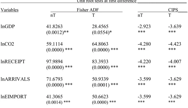
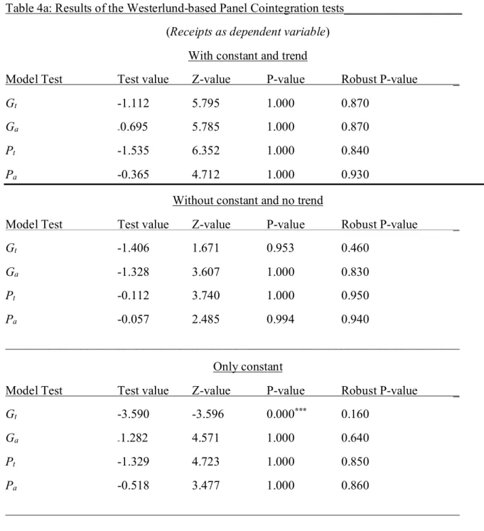
Given the result of the CD test by Pesaran (2004) which shows evidence of cross-section dependence, second generation panel models of Fisher-type ADF and the CIPS unit root results are provided in Table 2. Using a maximum lag of one at levels, both test models showed that all the variables are non-stationary by failing to reject the null hypothesis of unit root. But there is stationarity evidence even at 1% significance level when the tests are repeated at after first difference i.e I(1) with and without trend except for GDP that was stationary with trend at about 5%. Further unit root test by Hadri (2000) LM with results shown in Table 3 used a stationarity null hypothesis instead of the conventional unit root hypothesis of the earlier tests. The Hadri (2000) LM tests for the variables rejects stationarity null hypothesis with mean, demean, without trend, and trend without mean all at 1% statistical significance levels. The Tables 4 a & b present the results of cointegration test by Westerlund (2007) using maximum lag of one (1) based on AIC (Akaike’s Information Criterion). Given receipts as the dependent variable, the results show no evidence of cointegration both with constant and trend and without both in the
whole cross-section and time (Ga, Gt) sample and within the cross-section and time (Pa, Pt)
sample. But the case is different when only constant is applied; a t-value of -3.590 with P-value of 0.000 rejects the null hypothesis of no cointegration at statistical significant level of 1% for
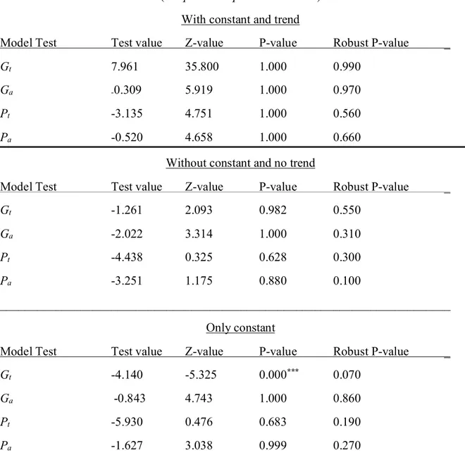
variable gives similar result as observed in Table 4b. In this case, also the null hypothesis of no cointegration of only Ga is rejected but with t-value of -4.140 and P-value of 0.000 (statistically significant at 1% level).
The results of the PMG estimation of the short-run and long-run coefficients of the
energy import (Eimport), arrivals, CO2 and GDP coefficients and the respective adjustment
coefficients (convergence parameter) are presented in Table 5. Estimating the cointegration equation using Pesaran et al. (1999) which is performed without trend, the adjustment coefficients that provide allowances from short-run to long-run are estimated considering the homogeneity among estimated variables across the countries. The magnitude of long-run Eimport elasticities for PMG and MG of -0.133 and 1.334 are respectively significant at 10% and no level of statistical significance. Specifically for the case of Eimport, the adjustment coefficients -0.190, -.426 and -0.154 respectively presents the short-run dynamics of PMG, MG and DFE that are all significant at 1% level. Since the PMG estimator ensures the inequality of the long-run elasticities across all panels as obvious in our estimate results, then the PMG approach is expected to yield efficient and consistent estimates.
Applying the specification Hausman test to appropriately by select between PMG and Mg yields a chi-squared test value of 2.35 with probability value of 0.3091. Also, since the P-value 0.3091 is greater than 0.05 i.e P-value: 0.309 > 0.05, the null hypothesis of PMG is not rejected. This implies that PMG approach is preferred.
4.2 Robustness Evidence
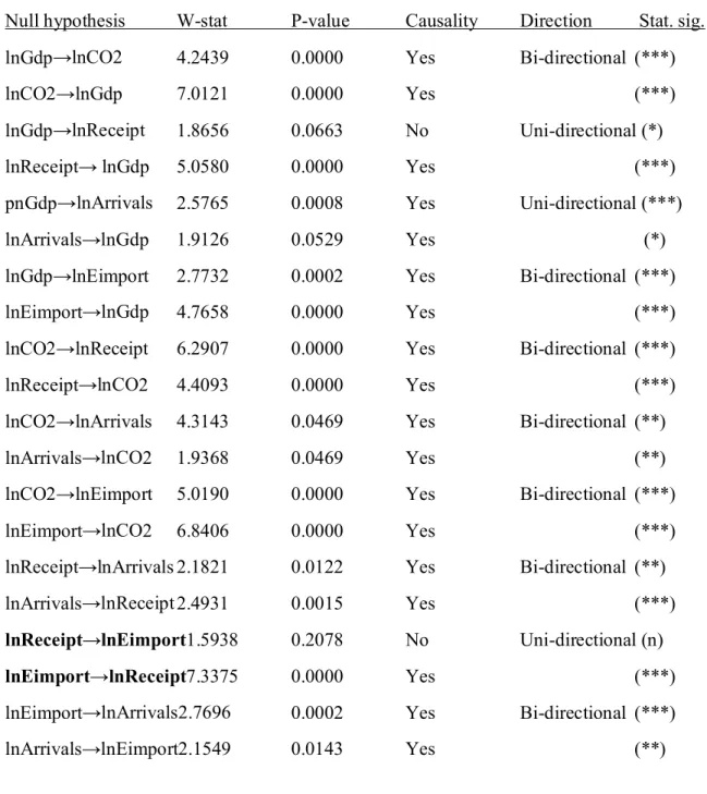
The Granger causality result of the Table 6 depicts a robustness test of the relationship between specifically receipts and Eimport and between other estimated variables. The result shows a
CO2 and arrivals, CO2 and Eimport, Receipts and arrivals, and Eimport and arrivals at 5% significance level by rejecting the null hypothesis of no Granger causality. But there exists evidence of one-directional Granger causality between Receipt and Eimport, GDP and receipts, and GDP and arrivals at 5% significance level. Specifically from the result, Eimport granger causes receipts implies that previous information on energy imports could be useful predictor of international tourism receipts across the panel of countries but the reverse is not true.
5. Concluding Remarks, Recommendation and Policy Implication
Most of the coastline Mediterranean countries are largely depending on energy importation to meet their respective domestic demands. This study investigates the long-run relationship between tourism receipts, energy import (component of good and services), a deviation from the normal trend of literature on tourism receipts concepts, and in relation to tourism arrival, carbon
emission (CO2) and GDP. Empirical evidence using the Pooled Mean Group by Pesaran et al.
(1999) to address the heterogeneity problems shows a weak long-run relationship between energy import and tourism receipts. Although, empirical evidences shows only strong long-run
equilibrium relationship between tourism receipts and tourism arrivals, CO2 and GDP which
were in line with results from previous literature (Alola & Alola, 2018), the result is different for energy import. For the tourism receipts and energy import nexus, short-run and long-run coefficients are negative in value, an unusual result that suggests a hint for more careful study and observation into tourism receipt-energy import nexus. The causality result shows seven (7) bi-directional relationships between estimated variables across the countries except from GDP to receipts, GDP to arrivals and Eimport to receipts that were uni-directional with the reverse cases not possible. However, the result of causality from Eimport to receipts agrees with the natural intuition.
5.1 Direction for Further Study
Further study of this conceived tourism-energy import concept is encouraged especially on a wider coverage as to ascertain possible impact and extent of impact among the duo. It is good to note that comprehensive analysis within this framework would require a study of tourism-energy import concept, detailing the types of energy sources, the composition of coastline Mediterranean Sea countries, and among other factors. However, the country-specific control of energy import which strongly depends on domestic energy needs and availability of domestic energy resources will require careful examination as per country natural resources distributional patterns and even global energy production among other factors over time.
5.2 Policy Implication
On policy implementation framework, energy import like importation of most good and services is expected to aid infrastructural, institutional, societal, cultural, and economic developments of a state. For the naturally tourist destination countries, the CMCs for instance, implementation of policies that could further aid sectoral developments and the expansion of the sector would be instrumental to enhancing the ready-made tourism market. Evidently, the result which indicate causality only from Eimport to receipts suggests that previous information of energy import is useful predictor of international tourism receipts in across the countries (the reverse is not true). But the cointegration results throws caution to suggest strategic policy is essential regarding the energy market in the region. The negative coefficient values from the short-run to long-run (the adjustment speed) of short-run dynamic of -0.1901493 further suggest energy import policies that are aimed at enhancing development of indigenous or domestic source of energy thereby sustaining an efficient tourism market. Also, the tools of international policy framework especially that is targeted at sustaining peace toward mitigating devastating effect caused by
regional unrest to energy import is essential. To neutralize these regional impacts caused mainly by incessant unrests in Libya, Iraq and other Middle East countries, international collaborations would be considered essential. More pertinent is that the height of insecurity around the region would not only hamper energy import, but potential tourist or visitors to the region would simply avoid the region. This is in line with the investigation of oil import and energy security concern raised by Vivoda (2009) while referencing the world's top three oil importers, the United States, Japan, and China.
5.2.1 Implication for Theory
Hospitality industry relies heavily on water, energy and other non-durable products for successful delivery of quality services thereby provoking a substantial impact on the environment. Interestingly, the core value of hospitality requires clean and unpolluted natural environment to thrive (Cingoski, & Petrevska, 2018). Thus, promoting sustainable environment is precursory to maintaining competitive advantage in the industry. Hence, tourism stakeholders especially hoteliers must embrace energy efficient and low-carbon technologies approach in their operations. Specifically, we advocate the use of renewable energy sources which will increase the supply of energy for hospitality operation and reduces over-reliance on energy imports. Shifting energy source is not only cost-effective for the business owner but also guarantees improved environmental quality necessary for maintaining their competitive edge in a volatile marketplace.
Governments of CMCs may also formulate and implement low-carbon economy policy that encourages hospitality state holders to incorporate sustainability to their operations thereby leading the way to the preservation of the environment, natural resources and the ecosystem by following a path that condenses environmental pollution and advance environmental quality.
Since tourism development is highly dependent on energy import, approaching sustainable tourism development through the implementation of renewable energy will also help in achieving the goal of balancing economic growth with adequate environmental quality. Government therefore are advised to create initiatives that provides incentives to business organizations that opt for application of low carbon technologies in their operations such as in transportation, accommodation, logistics and other services and/or tourism related operations in order to avoid overexploitation of the natural resources and minimizes carbon emission.
While in the short-run the associated cost of implementing low-carbon and renewable energy approach may seem expensive, the long-run benefits outweighs the cost as it guarantees sustainability of the business due to its compliance to the global trend on sustainable development and the increasing awareness of consumer to the importance of green initiatives.
Funding
I hereby declare that there is no form of funding received toward this study.
Compliance with Ethical Standards
The author wish to disclose here that there is no potential conflicts of interest at any level of this study
References
Akadiri, S. S., & Akadiri, A. C. (2019). Examining The Causal Relationship Between Tourism, Exchange Rate, And Economic Growth In Tourism Island States: Evidence From Second-Generation Panel. International Journal of Hospitality & Tourism Administration, 1-16. Akadiri, S. S., Akadiri, A. C., & Alola, U. V. (2017). Is there growth impact of tourism?
Al-mulali, U., Fereidouni, H. G., Lee, J. Y. M., & Mohammed, A. H. (2014). Estimating the tourism-led growth hypothesis: A case study of the Middle East countries. Anatolia, 25(2), 290-298. doi:10.1080/13032917.2013.843467.
Alola, A. A. (2019). Carbon emissions and the trilemma of trade policy, migration policy and health care in the US. Carbon Management, 10(2), 209-218.
Alola, A. A. (2019). The trilemma of trade, monetary and immigration policies in the United States: Accounting for environmental sustainability. Science of The Total Environment, 658, 260-267.
Alola, A. A., & Alola, U. V. (2018a). The Dynamics of Tourism—Refugeeism on House Prices in Cyprus and Malta. Journal of International Migration and Integration, 1-16.
Alola, A. A., & Alola, U. V. (2018b). Agricultural land usage and tourism impact on renewable energy consumption among Coastline Mediterranean Countries. Energy & Environment, 0958305X18779577.
Alola, A. A., Alola, U. V., Akadiri, S. S. (2019). Renewable energy consumption in Coastline Mediterranean Countries: Impact of environmental degradation and housing policy. (In Press).
Alola, A. A., Bekun, F. V., & Sarkodie, S. A. (2019). Dynamic impact of trade policy, economic growth, fertility rate, renewable and non-renewable energy consumption on ecological footprint in Europe. Science of The Total Environment, 685, 702-709.
Asafu-Adjaye, J. (2000). The relationship between energy consumption, energy prices and economic growth: time series evidence from Asian developing countries. Energy
economics, 22(6), 615-625.
Balli, E., Sigeze, C., Manga, M., Birdir, S., & Birdir, K. (2019). The relationship between tourism, CO2 emissions and economic growth: a case of Mediterranean countries. Asia
Becken, S., & Patterson, M. (2006). Measuring national carbon dioxide emissions from tourism as a key step towards achieving sustainable tourism. Journal of Sustainable Tourism, 14(4), 323-338.
Bekun, F. V., Alola, A. A., & Sarkodie, S. A. (2019). Toward a sustainable environment: Nexus between CO2 emissions, resource rent, renewable and nonrenewable energy in 16-EU countries. Science of the Total Environment, 657, 1023-1029.
Cingoski, V., & Petrevska, B. (2018). Making hotels more energy efficient: the managerial perception. Economic research-Ekonomska istraživanja, 31(1), 87-101.
Dritsakis, N. (2004). Tourism as a long-run economic growth factor: An empirical investigation for Greece using causality analysis. Tourism Economics, 10(3), 305-316.
Dumitrescu, E. I., & Hurlin, C. (2012). Testing for Granger non-causality in heterogeneous panels. Economic Modelling, 29(4), 1450-1460.
Gokmenoglu, K. K., & Eren, B. M. (2019). The role of international tourism on energy consumption: empirical evidence from Turkey. Current Issues in Tourism, 1-7.
Im, K. S., Pesaran, M. H., & Shin, Y. (2003). Testing for unit roots in heterogeneous panels.
Journal of Econometrics, 115(1), 53-74.
Johansen, S. (1988). Statistical analysis of cointegration vectors. Journal of Economic Dynamics
and Control, 12(2), 231-254.
Katircioglu, S. (2009). Tourism, trade and growth: the case of Cyprus. Applied
Economics, 41(21), 2741-2750.
Katircioglu, S., Cizreliogullari, M. N., & Katircioglu, S. (2019). Estimating the role of climate changes on international tourist flows: evidence from Mediterranean Island States.
Katircioglu, S., Gokmenoglu, K. K., & Eren, B. M. (2018). Testing the role of tourism development in ecological footprint quality: evidence from top 10 tourist destinations.
Environmental Science and Pollution Research, 25(33), 33611-33619.
Kilic, C., & Bayar, Y. (2014). Effects of real exchange rate volatility on tourism receipts and expenditures in turkey. Advances in Management and Applied Economics, 4(1), 89-101. Kwiatkowski, D., Phillips, P. C., Schmidt, P., & Shin, Y. (1992). Testing the null hypothesis of
stationarity against the alternative of a unit root: How sure are we that economic time series have a unit root? Journal of Econometrics, 54(1-3), 159-178.
Levin, A., Lin, C., & Chu, C. J. (2002). Unit root tests in panel data: Asymptotic and finite-sample properties. Journal of Econometrics, 108(1), 1-24.
Lee, J. W., & Brahmasrene, T. (2013). Investigating the influence of tourism on economic growth and carbon emissions: Evidence from panel analysis of the European Union. Tourism Management, 38, 69-76.Liu, J. C., & Var, T. (1986). Resident attitudes toward tourism impacts in hawaii. Annals of Tourism Research, 13(2), 193-214.
Maddala, G. S., & Wu, S. (1999). A comparative study of unit root tests with panel data and a new simple test. Oxford Bulletin of Economics and Statistics, 61(S1), 631-652.
Paramati, S. R., Alam, M. S., & Chen, C. (2016). The effects of tourism on economic growth and CO2 emissions A comparison between developed and developing economies. Journal of
Travel Research, , 0047287516667848.
Pesaran, M. H. (2004). General diagnostic tests for cross section dependence in panels.
Pesaran, M. H. (2007). A simple panel unit root test in the presence of cross‐section dependence. Journal of Applied Econometrics, 22(2), 265-312.
Proença, S., & Soukiazis, E. (2008). Tourism as an economic growth factor: a case study for Southern European countries. Tourism Economics, 14(4), 791-806.
Rauch, J. E., & Trindade, V. (2002). Ethnic Chinese networks in international trade. Review of
Economics and Statistics, 84(1), 116-130.
Raghoo, P., Surroop, D., Wolf, F., Leal Filho, W., Jeetah, P., & Delakowitz, B. (2018). Dimensions of energy security in small island developing states. Utilities Policy, 53, 94-101. Saint Akadiri, S., Alola, A. A., Akadiri, A. C., & Alola, U. V. (2019). Renewable energy consumption in EU-28 countries: policy toward pollution mitigation and economic sustainability. Energy Policy, 132, 803-810.
Saint Akadiri, S., Alola, A. A., & Akadiri, A. C. (2019). The role of globalization, real income, tourism in environmental sustainability target. Evidence from Turkey. Science of The Total
Environment.
Saint Akadiri, S., Lasisi, T. T., Uzuner, G., & Akadiri, A. C. (2019). Examining the impact of globalization in the environmental Kuznets curve hypothesis: the case of tourist destination states. Environmental Science and Pollution Research, 1-11.
Seetanah, B. (2011). Assessing the dynamic economic impact of tourism for island economies.
Annals of Tourism Research, 38(1), 291-308.
Shan, J., & Wilson, K. (2001). Causality between trade and tourism: Empirical evidence from china. Applied Economics Letters, 8(4), 279-283.
Tang, C. F., & Abosedra, S. (2014). Small sample evidence on the tourism-led growth
hypothesis in Lebanon. Current Issues in Tourism, 17(3), 234-246.
doi:10.1080/13683500.2012.732044
Tang, C. F., & Abosedra, S. (2016). Tourism and growth in lebanon: New evidence from bootstrap simulation and rolling causality approaches. Empirical Economics, 50(2), 679-696.
Tugcu, C. T. (2014). Tourism and economic growth nexus revisited: A panel causality analysis for the case of the Mediterranean Region. Tourism Management, 42, 207-212.
Üstün, Ç. (2011). Energy Cooperation between Import Dependent Countries: Cases of Italy and Turkey. Perceptions, 16(1), 71.
Vivoda, V. (2009). Diversification of oil import sources and energy security: A key strategy or an elusive objective? Energy Policy, 37(11), 4615-4623.
Wang, B., Wang, Q., Wei, Y. M., & Li, Z. P. (2018). Role of renewable energy in China’s
energy security and climate change mitigation: An index decomposition
analysis. Renewable and sustainable energy reviews, 90, 187-194.
Westerlund, J. (2007). Testing for error correction in panel data. Oxford Bulletin of Economics
and statistics, 69(6), 709-748.
Westerlund, J., & Edgerton, D. L. (2007). A panel bootstrap cointegration test. Economics
Letters, 97(3), 185-190.
Persyn, D., & Westerlund, J. (2008). Error-correction-based cointegration tests for panel data. Stata Journal, 8(2), 232-241.
World Tourism Organization. (2016). UNWTO tourism highlights. https://www.e-unwto.org/doi/book/10.18111/9789284418145.
World Tourism Organization. (2018). UNWTO tourism highlights
https://www.e-unwto.org/doi/book/10.18111/9789284419876
World Development Indicator (WDI, 2019). http://data.worldbank.org/data-catalog/world-development-indicators.
World Development Indicator (WDI, 2016). http://data.worldbank.org/data-catalog/world-development-indicators.
Wilson Center. (2015). Chapter 11 Update: Energy Security in the Mediterranean Region. Chapter 11
Update: Energy Security in the Mediterranean Region
Zhang, S., & Liu, X. (2019). The roles of international tourism and renewable energy in environment: New evidence from Asian countries. Renewable Energy, 139, 385-394.
Zhao, X., & Wu, Y. (2007). Determinants of China's energy imports: An empirical analysis. Energy Policy, 35(8), 4235-4246.
Table 1: Coastline Mediterranean countries energy import-tourism receipts for 2013 _
International tourism receipt Energy Import
Countries (% of total export) (% of total consumption______
Cyprus 94.35630779 21.56932204 Egypt 15.06188163 -6.813640123 France 7.871685166 46.21446763 Israel 7.124425886 73.09228372 Italy 7.124425886 76.3388121 Morocco 25.14533159 90.08664936 Spain 14.28759482 70.34306113 Tunisia 13.02769952 29.92229961 Turkey 16.68531861 72.23197311_______________
Note: The negative sign in value of energy import indicates no importation but rather exportation like the case of Egypt (a major crude oil producing country in the region.
Table 2: Panel unit root tests______________________________________________________ Unit root tests at level_____________________________
Variables Fisher ADF CIPS____
nT T nT T lnGDP 2.6471 9.4164 -1.164 -0.639 (1.0000) (0.9493) lnCO2 4.8221 6.8952 -0.559 -2.293 (0.9991) (0.9910) lnRECEIPT 9.1322 32.4514 -1.278 -2.789 (0.9566) (0.0194) lnARRIVALS 25.1529 27.3763 -1.981 -1.855 (0.1208) (0.0722) lnEIMPORT 15.4310 7.3073 -0.788 -2.109 (0.6322) (0.9873) ________________________________________________________________________________
Unit root tests at first difference _____________________
Variables Fisher ADF CIPS____
nT T nT T lnGDP 41.8263 28.4565 -2.923 -3.639 (0.0012)** (0.0554)* *** *** lnCO2 59.1114 64.8063 -4.280 -4.423 (0.0000) *** (0.0000) *** *** *** lnRECEIPT 97.9894 83.3933 -4.220 -4.007 (0.0000) *** (0.0000) *** *** *** lnARRIVALS 71.6793 50.9339 -3.599 -3.629 (0.0000) *** (0.0001) *** *** *** lnEIMPORT 41.3065 50.6623 -3.599 -3.629 (0.0014) *** (0.0000) *** *** *** ______________________________________________________________________________
Note: ***,** and *are statistical significance of the variable at 1%, 5% and 10% respectively. In this case the estimates above indicate statistical significance at 1% which means they are then significant at 5% and 10%. (Here, null hypothesis for stationarity are rejected in all cases using the estimated chi-values with p-values in parenthesis).
Table 3: Panel unit root tests_________________________________________________________ HADRI LM_______________________________ Variable M DM nT T+DM_________ lnGDP 14.6316*** 12.6949*** 5.6245 *** 6.4478 *** (0.0000) (0.0000) (0.0000) (0.0000) lnCO2 6.7279*** 7.8601 *** 12.1755*** 11.7744*** (0.0000) (0.0000) (0.0000) (0.0000) lnRECEIPT 13.4539*** 13.5261*** 7.9558 *** 6.3605 *** (0.000) (0.0000) (0.0000) (0.000) lnARRIVALS 15.3789*** 13.5081*** 8.0382 *** 8.5855 *** (0.000) (0.0000) (0.0000) (0.0000 lnEIMPORT 13.9778*** 14.6375*** 7.8452*** 4.5668 *** (0.000) (0.0000) (0.0000) (0.0000) ______________________________________________________________________________
Note: ***,** and *are statistical significance of the variable at 1%, 5% and 10% respectively. In this case the estimates above indicate statistical significance at 1% which means they are then significant at 5% and 10%. (Here, null hypothesis for stationarity are rejected in all cases using the estimated chi-values with p-values in parenthesis). M, Dm, nT and T+Dm are estimates with Mean, Demean, No Trend, and Trend and Demean respectively.
Table 4a: Results of the Westerlund-based Panel Cointegration tests___________________ (Receipts as dependent variable)
With constant and trend
Model Test Test value Z-value P-value Robust P-value _
Gt -1.112 5.795 1.000 0.870
Ga -0.695 5.785 1.000 0.870
Pt -1.535 6.352 1.000 0.840
Pa -0.365 4.712 1.000 0.930
Without constant and no trend
Model Test Test value Z-value P-value Robust P-value _
Gt -1.406 1.671 0.953 0.460 Ga -1.328 3.607 1.000 0.830 Pt -0.112 3.740 1.000 0.950 Pa -0.057 2.485 0.994 0.940 _________________________________________________________________________ Only constant
Model Test Test value Z-value P-value Robust P-value _
Gt -3.590 -3.596 0.000*** 0.160
Ga -1.282 4.571 1.000 0.640
Pt -1.329 4.723 1.000 0.850
Pa -0.518 3.477 1.000 0.860
Table 4b: Results of the Westerlund-based Panel Cointegration tests___________________ (Eimport as dependent variable)
With constant and trend
Model Test Test value Z-value P-value Robust P-value _
Gt 7.961 35.800 1.000 0.990
Ga -0.309 5.919 1.000 0.970
Pt -3.135 4.751 1.000 0.560
Pa -0.520 4.658 1.000 0.660
Without constant and no trend
Model Test Test value Z-value P-value Robust P-value _
Gt -1.261 2.093 0.982 0.550 Ga -2.022 3.314 1.000 0.310 Pt -4.438 0.325 0.628 0.300 Pa -3.251 1.175 0.880 0.100 _________________________________________________________________________ Only constant
Model Test Test value Z-value P-value Robust P-value _
Gt -4.140 -5.325 0.000*** 0.070
Ga -0.843 4.743 1.000 0.860
Pt -5.930 0.476 0.683 0.190
Pa -1.627 3.038 0.999 0.270
_________________________________________________________________________
Note: *** indicates 1% statistical significance level. Maximum lag selection by AIC of lag one (1) is used and the Bartlett kernel window width set to 4(T/100)2/9 ≈ 3.
Table 5: Pooled Mean and Mean Group (PMG & MG) and DFE test results_____________
Convergence Long-run Short-run Hausman
Model Test parameter coefficient coefficient test _
MG -.4260055 1.336254 -0.880261 (0.000) *** (0.167) (0.210) DFE -0.1535229 -0.4442473 -0.0000588 (0.000) *** (0.036) ** (0.999) PMG -0.1901493 -0.13271 -0.2705003 2.35 Eimport (0.004) *** (0.079) * (0.320) (0.3091) -0.1901493 -9.289091 -0.200485 CO2 (0.004) *** (0.001) *** (0.867) -0.1901493 -.0023407 0.0002726 GDP (0.004) *** (0.000) *** (0.546) 0.1901493 1.12e-06 8.15e-07 ARRIVALS (0.004) *** (0.000) *** (0.122)
Table 6: Panel Granger causality results by Dumitrescu and Hurlin (2012)______________
Null hypothesis W-stat P-value Causality Direction Stat. sig.
lnGdp→lnCO2 4.2439 0.0000 Yes Bi-directional (***)
lnCO2→lnGdp 7.0121 0.0000 Yes (***)
lnGdp→lnReceipt 1.8656 0.0663 No Uni-directional (*)
lnReceipt→ lnGdp 5.0580 0.0000 Yes (***)
pnGdp→lnArrivals 2.5765 0.0008 Yes Uni-directional (***)
lnArrivals→lnGdp 1.9126 0.0529 Yes (*)
lnGdp→lnEimport 2.7732 0.0002 Yes Bi-directional (***)
lnEimport→lnGdp 4.7658 0.0000 Yes (***)
lnCO2→lnReceipt 6.2907 0.0000 Yes Bi-directional (***)
lnReceipt→lnCO2 4.4093 0.0000 Yes (***)
lnCO2→lnArrivals 4.3143 0.0469 Yes Bi-directional (**)
lnArrivals→lnCO2 1.9368 0.0469 Yes (**)
lnCO2→lnEimport 5.0190 0.0000 Yes Bi-directional (***)
lnEimport→lnCO2 6.8406 0.0000 Yes (***)
lnReceipt→lnArrivals 2.1821 0.0122 Yes Bi-directional (**)
lnArrivals→lnReceipt 2.4931 0.0015 Yes (***)
lnReceipt→lnEimport1.5938 0.2078 No Uni-directional (n)
lnEimport→lnReceipt7.3375 0.0000 Yes (***)
lnEimport→lnArrivals2.7696 0.0002 Yes Bi-directional (***)
lnArrivals→lnEimport2.1549 0.0143 Yes (**)
-80 -40 0 40 80 120 1 9 5 1 0 1 1 0 7 1 1 3 2 0 0 2 0 6 2 1 2 3 9 9 3 0 5 3 1 1 4 9 8 4 0 4 4 1 0 5 9 7 5 0 3 5 0 9 6 9 6 6 0 2 6 0 8 7 9 5 7 0 1 7 0 7 7 1 3 8 0 0 8 0 6 8 1 2 9 9 9 9 0 5 9 1 1 RECEIPTS E-IMPORT
Figure 1: The graph showing the co-movement of tourism receipts and energy import across the countries over time. Note: Eimport is the trend above while receipts is mostly beneath.
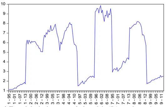
1 2 3 4 5 6 7 8 9 10 1 9 5 1 0 1 1 0 7 1 1 3 2 0 0 2 0 6 2 1 2 3 9 9 3 0 5 3 1 1 4 9 8 4 0 4 4 1 0 5 9 7 5 0 3 5 0 9 6 9 6 6 0 2 6 0 8 7 9 5 7 0 1 7 0 7 7 1 3 8 0 0 8 0 6 8 1 2 9 9 9 9 0 5 9 1 1 CO2
0 10,000 20,000 30,000 40,000 50,000 1 9 5 1 0 1 1 0 7 1 1 3 2 0 0 2 0 6 2 1 2 3 9 9 3 0 5 3 1 1 4 9 8 4 0 4 4 1 0 5 9 7 5 0 3 5 0 9 6 9 6 6 0 2 6 0 8 7 9 5 7 0 1 7 0 7 7 1 3 8 0 0 8 0 6 8 1 2 9 9 9 9 0 5 9 1 1 GDP
Figure 3: The graph showing the movement of GDP across the countries over time
0 10,000,000 20,000,000 30,000,000 40,000,000 50,000,000 60,000,000 70,000,000 80,000,000 90,000,000 1 9 5 1 0 1 1 0 7 1 1 3 2 0 0 2 0 6 2 1 2 3 9 9 3 0 5 3 1 1 4 9 8 4 0 4 4 1 0 5 9 7 5 0 3 5 0 9 6 9 6 6 0 2 6 0 8 7 9 5 7 0 1 7 0 7 7 1 3 8 0 0 8 0 6 8 1 2 9 9 9 9 0 5 9 1 1 ARRIVALS
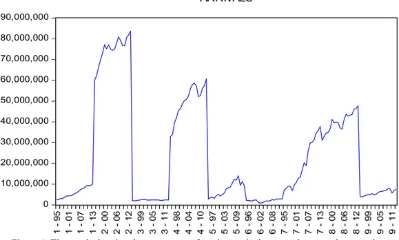
Figure 4: The graph showing the movement of tourism arrivals across the countries over time