sustainability
ArticleIn the Presence of Climate Change, the Use of
Fertilizers and the Effect of Income on
Agricultural Emissions
Bahar Celikkol Erbas1,† ID and Ebru Guven Solakoglu2,*,†
1 Department of Economics, TOBB University of Economics and Technology, Ankara 06530, Turkey; [email protected]
2 Banking and Finance, Bilkent University, Ankara 06800, Turkey * Correspondence: [email protected]; Tel.: +90-312-290-1138
† Authors are listed in the alphabetical order and share the contributions equally. Received: 21 July 2017; Accepted: 24 October 2017; Published: 31 October 2017
Abstract:This study looks into the factual link between nitrogen fertilizer use and the land annual mean temperature anomalies arising from climate change, incorporating the effect of income and agriculture share to understand better their impact on emissions from agricultural activities along climate indicators. The study unearths causalities associated with this link by employing the Vector Error Correction Model (VECM) with back-dated actual panel data specifically constructed for this study by combining four datasets from 2002 to 2010. In the long-run, the causality is significant and unidirectional, indicating that income, agriculture share, and land temperature anomalies cause agricultural emissions, and that disequilibrium from such emissions is not eliminated within a year. In the short-run, the effective use of nitrogen fertilizers and other associated agricultural practices can be achieved as countries approach per capita income of 7000 USD. Changes in the structure of economies have an expected effect on agricultural emissions. Temperature anomalies increase agricultural emissions from nitrogen fertilizers, possibly due to the fact that the potential negative impacts of these anomalies are mitigated by farmers through changes in crop production inputs. Therefore, as part of adoption strategies, to avoid the excessive and inefficient use of nitrogen fertilizers by farmers, economic incentives should be aligned with the national and global incentives of sustainability.
Keywords:agriculture; nitrogen fertilizer; climate change; VECM
JEL Classification:Q10; Q53; Q54; Q56
1. Introduction
In the face of global warming, agricultural production systems must become more resilient to long-term changes in temperature and precipitation, as well as to disruptive events. By the year 2100, under different scenarios, climate change is predicted to have an impact on the market (as a percent of GDP) for the entire world—but more so for poorer countries than for richer ones. Agriculture, as a climate sensitive sector, plays an important role in the economies of poor countries, where the impact is larger and the relationship between crop responses and temperature follows an inverted U-shape relationship [1]. Changes in crop yields, in turn, might affect the use of agricultural inputs, including nitrogen fertilizer. The resilience of agricultural production systems to climate change requires higher efficiency in the use of natural resources and inputs of agricultural production [2]. In order to employ agricultural inputs more efficiently in the production process and thus adopt less
Sustainability 2017, 9, 1989 2 of 17
emission intensive technologies, the effects of climate change on the use of these inputs need to be understood better.
The literature presents experimental and cross-sectional studies on the impact of future climate scenarios in five sectors, namely, water, energy, timber, coasts, and agriculture, as well as in the economy overall [1]. Moreover, the literature shows global and country-level specific studies investigating crop-switching, the Ricardian method, and temperature affects under future climate scenarios [3–5]. Zinyengere, Crespo and Hachigonta [6] and Chen et al. [7] provide extensive literature reviews on crop-response projections for South Africa and China, respectively. Existing studies with the Ricardian method assume that farmers alter their inputs, outputs, and practices in response to climate change [3]. Furthermore, a field survey from China reveals that, when faced with drought, in order to mitigate the potential negative impacts, 35 percent of farmers in China change crop production inputs (e.g., seeds, fertilizer, pesticides, and labor) and 24 percent of farmers adjust crop planting and/or harvesting time [8].
Although there is a significant body of literature in the science domain at all scales and in economics at the micro level, empirical studies at the global scale on the linkage of economic development with fertilizer use and agricultural emissions based on actual or historical data are underprovided [9,10].
While the change in the amount of nitrogen fertilizer consumed might help farmers to adapt to global warming, this change in and of itself alters nitrous oxide emissions from agriculture. Therefore, studying these effects at a more macro level with actual country-level historical data would provide evidence for targeted mitigation efforts and options for adaptation.
As an indirect energy, fertilizer plays an important role in maintaining soil fertility and hence in increasing crop yields, which is the most important source of growth in crop production, followed closely by expanding land area and increasing the frequency of harvest. Thus, the role of fertilizer in feeding the world is not disputable. As more countries become further developed, and as the size of the world population increases, the demand for agricultural output will continue to grow. At the same time, responsible policies that predict environmental quality will evolve in the presence of global warming. The effects of economic growth on various dimensions of environmental quality are analyzed using the environmental Kuznets curve (EKC) model. According to this approach, in the early stages of industrialization of a nation or clan, people give a higher priority to income than to the environment. As incomes rise, however, people are willing to pay for a cleaner environment more than for an increase in income. Thus, people accept and begin to welcome regulations imposed by institutions, and hence emission levels start to decline. Since the early 1990s, a few theoretical models have been introduced [11] as to why and how EKC appears, while more empirical studies have also been conducted [12]. Initial work in the literature has looked at this simple relationship, in order to understand whether economic growth along with trade influence are answers to environmental quality and how various people have supported this relationship.
The first generation of studies uses different indicators and draws different conclusions, but many empirically support an inverted-U shaped relationship. Grossman and Krueger [13] segregate the economic activity into scale, composition effects, and a shift in production techniques. The first two positively and ambiguously affect CO2emissions from economic activities, whereas the latter can be seen as a reason to decrease these emissions. Many theoretical papers have followed Grossman and Krueger [11,14,15]. Later works question the sensitivity of the relationship, depending on the methodology chosen in these empirical studies [16–21]. They use various sample countries and time periods and consider various types of pollutants. Most support the inverted-U shaped relationship of economic growth and CO2emissions, although their results differ in terms of the actual turning point. This second generation of arguments circles around two notions: the functional forms of the models and their environmental quality representations. Assumed functional forms, such as quadratic (U-shape) or cubic (N-shape) functions of income explaining CO2emissions, have been criticized by many [22–25]. Furthermore, some studies have drawn attention to the feedback of CO2
Sustainability 2017, 9, 1989 3 of 17
emissions on income as a problem of endogeneity [26,27] emphasizing the need for research on more complex bi-directional relationships between economic development and environmental quality as well as exactly how the demand for environmental quality should be measured. On the one hand, many studies introduce factors such as trade and openness [28]; distinguishing composition and scale effects [29]; incorporating property rights using the ratio of credit allocation to the private sector as a percentage of GDP [30]; energy use [31]; and land and quality of institutions [32] to explain environmental degradation. On the other hand, several other studies have more recently used different indicators for dependent variables of environmental degradation, such as ecological footprints [33,34] and environmental quality [35,36].
Recent studies suggest that the variables in the EKC model can often be integrated (non-stationary). However, early work on the EKC has not specifically looked into the time series structure of the data. This suggests that their results may be spurious and hence may have indicated incorrect EKC turning points. More recent studies have looked into the causal relationship between income and CO2and SO2 emissions by including energy consumption in their models [6,32,37,38].
Since the literature establishes the relationship between income and CO2and SO2via EKC, and since the EKC may provide an assessment of emission sustainability, although insufficient, we would like to leverage this paper’s questions within the EKC framework. While this study also tests for EKC, it differs from previous literature in three ways. First, we specify the N2O emission within the agricultural sector and focus on the use of nitrogen fertilizer. By doing so, we incorporate indirect energy consumption in the farming industry and segregate the emissions coming from farm-side food production that is essential for a fast-growing population. In other words, we integrate the environmental effects from agriculture and related energy use into the EKC approach in order to understand the mitigating and increasing effect of agricultural emissions within economic growth. Second, we acknowledge the causal effect between economic growth and agricultural emissions by using a cointegration technique and applying VECM to indicate short- and long-run effects. Third, we incorporate land annual mean temperature in the simple EKC model to control the effect of weather anomalies on nitrogen fertilizer use, also being aware of a possible bi-directional effect between them. The Role of Nitrogen Fertilizer Use
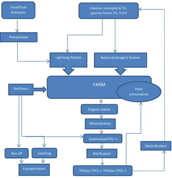
As the population grows and per capita consumption patterns change, farmers alter food, feed, livestock, and fiber production as well as energy use, land-use composition, and social equity [39]. All these changes, in turn, require use of nitrogen fertilizers. Erisman [40] indicates that the availability of synthetic fertilizers enables an increase in food production responsible for feeding about half of the current human population. Nitrogen (N) plays an important role in controlling a species’ diversity as well as the dynamics and functioning of many terrestrial, fresh water, and marine ecosystems. While added nitrogen is required to achieve higher crop yields, excessive use of nitrogen-enriched fertilizers causes environmental damage [41]. Because of the extensive use of fertilizer and pesticides, the production of crops and livestock is the main source of water pollution. Nitrogen fertilizers also contribute to global greenhouse gas emissions (GHG), as they are one of the major anthropogenic sources of nitrous oxide (N2O). Further, fertilizers also impact fishery and forestry. The nitrogen biogeochemical cycle (see Figure1) is the basis for understanding the importance of nitrogen fertilizer use and its environmental damage in agriculture [42,43].
The global cycle of nitrogen has been substantially altered by human activities, with the combustion of fossil fuels and agriculture. Vitousek et al. [43] summarize that such alteration has certainly been responsible for the following: (i) doubling the rate of nitrogen input into the terrestrial nitrogen cycle; (ii) increasing the global concentration of N2O, a potent GHG, as well as other nitrogen oxides; (iii) causing loss of soil nutrients that are vital for the long-term fertility of soil; (iv) acidifying soil, streams, and lakes in various regions; and (v) increasing the transfer of nitrogen via rivers to coastal oceans and estuaries.
Sustainability 2017, 9, 1989 4 of 17 Sustainability 2017, 9, 1989 4 of 17 Fossil/Fuel Emissions Gaseous atmospheric N2; gaseous losses (N2, N2O)
Precipitation Fertilizers Bacteria(nitrogen) fixation
FARM
Lightning fixation Organic matter Mineralization Ammonium(NH4+) NitrificationNitrites (NO2-); Nitrates (NO3-)
Plant consumption Leaching Run off Eutrophication Denitrification
Figure 1. Nitrogen cycle.
This paper adds to the breadth of existing literature by examining empirically the impact of both climate change and income on the agricultural emissions produced by the use of nitrogen fertilizer. Section 2 describes the EKC model, data description and methodology. Section 3 presents the empirical results. Section 4 concludes the study with discussion and suggestions for future research. 2. Model, Data and Methodology
We use a simple quadratic form of the EKC model, with environmental controls added subsequently. The first model asserts that the CO2 equivalent of N2O GHG emissions in the
agricultural sector (AgEm) depends on GDP per capita (GDPcap) and agricultural share in GDP (AgGDP), with error ε, time t, and country i.
it
AgGDP
3
it
2
GDPcap
2
it
GDPcap
1
it
AgEm
=
α
+
β
+
β
+
β
+
ε
(1)The model (1) is in the form of the relationship between environmental and economic growth. The dependent variable, an environmental indicator, is provided from the Food and Agricultural Organization’s Agri-Environmental Indicators (FAOSTAT) [44]. Under the categories of agri-environmental factors, we use data for the aggregated GHG emissions for N2O from agriculture. Data
is shown in total amounts in Gg CO2 eq and as a percentage share on the total GHG emissions from
the agricultural sector. The FAOSTAT agri-environmental dataset contains nine years of agricultural Figure 1.Nitrogen cycle.
This paper adds to the breadth of existing literature by examining empirically the impact of both climate change and income on the agricultural emissions produced by the use of nitrogen fertilizer. Section2describes the EKC model, data description and methodology. Section3presents the empirical results. Section4concludes the study with discussion and suggestions for future research.
2. Model, Data and Methodology
We use a simple quadratic form of the EKC model, with environmental controls added subsequently. The first model asserts that the CO2equivalent of N2O GHG emissions in the agricultural sector (AgEm) depends on GDP per capita (GDPcap) and agricultural share in GDP (AgGDP), with error ε, time t, and country i.
AgEmit=α+β1GDPcapit+β2GDPcap2it+β3AgGDP+εit (1) The model (1) is in the form of the relationship between environmental and economic growth. The dependent variable, an environmental indicator, is provided from the Food and Agricultural Organization’s Agri-Environmental Indicators (FAOSTAT) [44]. Under the categories of agri-environmental factors, we use data for the aggregated GHG emissions for N2O from agriculture. Data is shown in total amounts in Gg CO2eq and as a percentage share on the total GHG emissions from the agricultural sector. The FAOSTAT agri-environmental dataset contains nine years of agricultural emissions data
Sustainability 2017, 9, 1989 5 of 17
from 145 countries. Although the dataset lists 239 countries, some provide either no information or few years of information. Countries with less than 5 years of data were excluded. For total amounts of GgCO2eq, the excluded countries presented an average of 100, whereas the model data average is more than 8000.
As an independent variable, we use GDP per capita, obtained from the World Bank development indicators (WDI) database [45]. The model asserts a quadratic form of EKC. We also include the share of agricultural sector in GDP from the WDI database to incorporate the level of agricultural activities in various economies. In addition to the GDP per capita, the EKC studies include other variables that are influential on environmental degradation. In this context, the share of the agricultural sector can be used as a control variable, by means of its impact on fertilizer use. In the model (1) t stands for time and i represents a country. The parameters β are to be estimated from data, where β1< 0 and β2> 0 indicates an inverted-U shaped relationship between income and environment. In parallel to the literature [9], we expect to see a β3> 0, suggesting that if a country has a higher agriculture share in GDP, the fertilizer use will also be higher.
2.1. Fertilizer Use
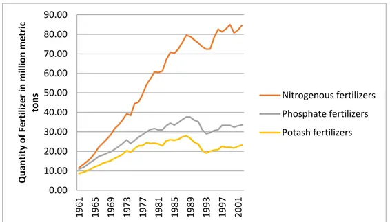
Figure2shows world nitrogen fertilizer consumption from 1961 to 2001, obtained from FAOSTAT under the measure of archived fertilizer data. [44] The use of each of the three fertilizers has increased considerably over the 40-year period, especially for nitrogenous fertilizers. Furthermore, while the use of phosphate and potash fertilizers has stabilized, especially in the last 20 years, the use of nitrogenous fertilizer continues to increase. Figure2shows a declining trend in the mid-1990s, corresponding to global economic problems in general and changes in Central Europe and the Former Soviet Union in particular [46].
When the use of fertilizer data is combined with agricultural yield and population data, it is observed that, unlike the other two fertilizers and yield, per capita nitrogenous fertilizer use has increased. The gap between the use of nitrogenous fertilizer and the other two fertilizers widens as a sluggish increase in yield is suppressed by a larger increase in fertilizer use. Because FAO [47] states that fertilizer use from agri-environmental and archived data should not be combined, Figures3and4 separate the data for approximately the same time period. We present the data only to understand better the behavior of nitrogen fertilizer use in the last half of the 20th century.
Sustainability 2017, 9, 1989 5 of 17
emissions data from 145 countries. Although the dataset lists 239 countries, some provide either no information or few years of information. Countries with less than 5 years of data were excluded. For total amounts of GgCO2 eq, the excluded countries presented an average of 100, whereas the model
data average is more than 8000.
As an independent variable, we use GDP per capita, obtained from the World Bank development indicators (WDI) database. [45] The model asserts a quadratic form of EKC. We also include the share of agricultural sector in GDP from the WDI database to incorporate the level of agricultural activities in various economies. In addition to the GDP per capita, the EKC studies include other variables that are influential on environmental degradation. In this context, the share of the agricultural sector can be used as a control variable, by means of its impact on fertilizer use. In the model (1) t stands for time and i represents a country. The parameters β are to be estimated from data, where β1 < 0 and β2
> 0 indicates an inverted-U shaped relationship between income and environment. In parallel to the literature [9], we expect to see a β3 > 0, suggesting that if a country has a higher agriculture share in
GDP, the fertilizer use will also be higher.
2.1. Fertilizer Use
Figure 2 shows world nitrogen fertilizer consumption from 1961 to 2001, obtained from FAOSTAT under the measure of archived fertilizer data. [44] The use of each of the three fertilizers has increased considerably over the 40-year period, especially for nitrogenous fertilizers. Furthermore, while the use of phosphate and potash fertilizers has stabilized, especially in the last 20 years, the use of nitrogenous fertilizer continues to increase. Figure 3 and 4 shows a declining trend in the mid-1990s, corresponding to global economic problems in general and changes in Central Europe and the Former Soviet Union in particular [46].
When the use of fertilizer data is combined with agricultural yield and population data, it is observed that, unlike the other two fertilizers and yield, per capita nitrogenous fertilizer use has increased. The gap between the use of nitrogenous fertilizer and the other two fertilizers widens as a sluggish increase in yield is suppressed by a larger increase in fertilizer use. Because FAO [47] states that fertilizer use from agri-environmental and archived data should not be combined, Figures 3 and 4 separate the data for approximately the same time period. We present the data only to understand better the behavior of nitrogen fertilizer use in the last half of the 20th century.
Figure 2. Fertilizer Consumption in the World.
0.00 10.00 20.00 30.00 40.00 50.00 60.00 70.00 80.00 90.00 19 61 19 65 19 69 19 73 19 77 19 81 19 85 19 89 19 93 19 97 20 01 Quantity of Fertilizer in million metric tons Nitrogenous fertilizers Phosphate fertilizers Potash fertilizers
Sustainability 2017, 9, 1989 6 of 17
Sustainability 2017, 9, 1989 6 of 17
Figure 3. Fertilizer use—yield relationship at level.
Figure 4. Fertilizer use—yield relationship at share. 2.2. Greenhouse Gas Emissions from Agriculture
FAOSTAT measures consist of the non-CO2 gases methane and nitrous oxide, produced by
aerobic and anaerobic decomposition processes in crop and livestock production and in management activities. We use the total amounts of nitrous oxide emissions in the agricultural sector as a Gg CO2
equivalent.
Figure 5 demonstrates the relationship between the agricultural emissions and GDP per capita. We segregate the level of GDP per capita according to the World Bank country classification. Figure 5 shows that, when moving from lower to higher income countries, GHG emissions from the agriculture sector follow a shape that is close to an inverted-U, similar to observations in the EKC literature. The highest level of GHG emissions from the agricultural sector is reached when countries have a medium level of income.
Similarly, moving from countries with higher levels of GDP per capita to those with lower levels, countries are placed somewhat on an inverted-U shape. The obvious pattern can be seen in Figure 6 for countries which have a greater than 25 percent agricultural share in GDP. The curve also shows a steep increase in the log of agricultural emissions for lower income countries. The countries with an agricultural share of 15 to 25 percent show high levels of agricultural emissions when compared to
15.00 15.50 16.00 16.50 17.00 17.50 18.00 18.50 19.00 19 61 19 65 19 69 19 73 19 77 19 81 19 85 19 89 19 93 19 97 20 01 quantity of fertilizers and yield in log terms Nitrogenous fertilizers Phosphate fertilizers Potash fertilizers Yield (Hg/100Ha) 0.0000 0.0020 0.0040 0.0060 0.0080 0.0100 0.0120 0.0140 0.0160 0.0180 19 61 19 64 19 67 19 70 19 73 19 76 19 79 19 82 19 85 19 88 19 91 19 94 19 97 20 00
share of fertilizers and yield
Nitrogenous fertilizers/ population Phosphate fertilizers/ population Potash fertilizers/ population Yield(Hg/100Ha)/ population Figure 3.Fertilizer use—yield relationship at level.
Sustainability 2017, 9, 1989 6 of 17
Figure 3. Fertilizer use—yield relationship at level.
Figure 4. Fertilizer use—yield relationship at share. 2.2. Greenhouse Gas Emissions from Agriculture
FAOSTAT measures consist of the non-CO2 gases methane and nitrous oxide, produced by
aerobic and anaerobic decomposition processes in crop and livestock production and in management activities. We use the total amounts of nitrous oxide emissions in the agricultural sector as a Gg CO2
equivalent.
Figure 5 demonstrates the relationship between the agricultural emissions and GDP per capita. We segregate the level of GDP per capita according to the World Bank country classification. Figure 5 shows that, when moving from lower to higher income countries, GHG emissions from the agriculture sector follow a shape that is close to an inverted-U, similar to observations in the EKC literature. The highest level of GHG emissions from the agricultural sector is reached when countries have a medium level of income.
Similarly, moving from countries with higher levels of GDP per capita to those with lower levels, countries are placed somewhat on an inverted-U shape. The obvious pattern can be seen in Figure 6 for countries which have a greater than 25 percent agricultural share in GDP. The curve also shows a steep increase in the log of agricultural emissions for lower income countries. The countries with an agricultural share of 15 to 25 percent show high levels of agricultural emissions when compared to
15.00 15.50 16.00 16.50 17.00 17.50 18.00 18.50 19.00 19 61 19 65 19 69 19 73 19 77 19 81 19 85 19 89 19 93 19 97 20 01 quantity of fertilizers and yield in log terms Nitrogenous fertilizers Phosphate fertilizers Potash fertilizers Yield (Hg/100Ha) 0.0000 0.0020 0.0040 0.0060 0.0080 0.0100 0.0120 0.0140 0.0160 0.0180 19 61 19 64 19 67 19 70 19 73 19 76 19 79 19 82 19 85 19 88 19 91 19 94 19 97 20 00
share of fertilizers and yield
Nitrogenous fertilizers/ population Phosphate fertilizers/ population Potash fertilizers/ population Yield(Hg/100Ha)/ population
Figure 4.Fertilizer use—yield relationship at share. 2.2. Greenhouse Gas Emissions from Agriculture
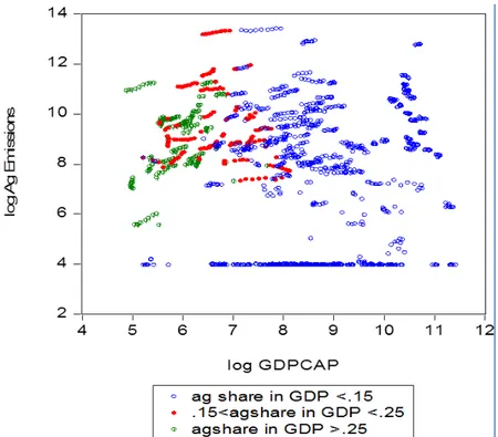
FAOSTAT measures consist of the non-CO2gases methane and nitrous oxide, produced by aerobic and anaerobic decomposition processes in crop and livestock production and in management activities. We use the total amounts of nitrous oxide emissions in the agricultural sector as a Gg CO2equivalent. Figure5demonstrates the relationship between the agricultural emissions and GDP per capita. We segregate the level of GDP per capita according to the World Bank country classification. Figure5 shows that, when moving from lower to higher income countries, GHG emissions from the agriculture sector follow a shape that is close to an inverted-U, similar to observations in the EKC literature. The highest level of GHG emissions from the agricultural sector is reached when countries have a medium level of income.
Similarly, moving from countries with higher levels of GDP per capita to those with lower levels, countries are placed somewhat on an inverted-U shape. The obvious pattern can be seen in Figure6 for countries which have a greater than 25 percent agricultural share in GDP. The curve also shows a steep increase in the log of agricultural emissions for lower income countries. The countries with an agricultural share of 15 to 25 percent show high levels of agricultural emissions when compared to
Sustainability 2017, 9, 1989 7 of 17
the rest of the data, but do not show a regular pattern within the group of countries. The countries with an agricultural share of less than 15 percent show more disputable behavior, unless we ignore the outliers of the countries with very low agricultural emissions or with very high income along with very high emissions. If these countries are counted as outliers and ignored, an inverted-U shape pattern can be observed from this presentation of data [32].
Figure 5. Relating economic growth with GHG emissions controlling income levels (with confidence area).
Figure 6. Relating the economic growth with GHG emissions controlling agricultural shares.
6 7 8 9 10 11 12 13 14 4 5 6 7 8 9 10 11 12 13 log of GDP per capita
log of A g E m issi ons
high income contries
medium-high income countries medium-low income countries lower income countries
Figure 5.Relating economic growth with GHG emissions controlling income levels (with confidence area).
Sustainability 2017, 9, 1989 7 of 17
the rest of the data, but do not show a regular pattern within the group of countries. The countries with an agricultural share of less than 15 percent show more disputable behavior, unless we ignore the outliers of the countries with very low agricultural emissions or with very high income along with very high emissions. If these countries are counted as outliers and ignored, an inverted-U shape pattern can be observed from this presentation of data [32].
Figure 5. Relating economic growth with GHG emissions controlling income levels (with confidence area).
Figure 6. Relating the economic growth with GHG emissions controlling agricultural shares.
6 7 8 9 10 11 12 13 14 4 5 6 7 8 9 10 11 12 13 log of GDP per capita
log of A g E m issi ons
high income contries
medium-high income countries medium-low income countries lower income countries
Sustainability 2017, 9, 1989 8 of 17
2.3. Climate—Temperature Anomalies
Before conveying the methodology of our analyses, we add another variable to our model to control altered anomalies in temperature changes. Shifts in climate may reduce food supplies and lead to a potential increase in malnutrition [48–51] and may increase crop vulnerability (though some regions may benefit from global climate change in the short run). Porter, J. R. et al. [52] show that climate attribution is increasingly documented not only for average conditions over crop growing seasons but also for extremes. More specifically, an increase in frequency of unusually hot nights, attributable to human activity, is found to be damaging to most crops and particularly observed for rice yields [53–55]. In addition, extreme high daytime temperatures are found to be damaging and sometimes lethal to crops on a global scale [56,57]. At both the regional and local level, it is important to note that soil temperature scales, soil moisture, and clouds each have a significant role in driving the trend sterns in daytime maximum temperature than the GHG emissions. Therefore, it is harder to attribute these trends to GHG emissions [58,59]. The scope of this study is global; therefore, the land annual mean temperature anomalies variable is added to the model as a control variable to capture the effect of the climate as much as possible. The addition of this environmental control variable may lessen the effect of omitted variable bias, leading to a possible endogeneity problem. Model (2) includes this variable.
AgEmit =α+β1GDPcapit+β2GDPcap2it+β3AgGDP+β4WA+εit (2)
We incorporated the National Aeronautics and Space Administration (NASA) Goddard Institute for Space Studies’ (GISS) zonal annual means data [60] to our main dataset. The National Oceanic and Atmospheric Administration’s (NOAA) National Climatic Data Center (NCDC) [61] states that surface temperature anomalies’ data are useful as a global-scale climate diagnostic tool and provide an overview of mean global temperatures, when compared to a reference value. Since anomaly data is used to investigate regional and global patterns and to provide temperature information with respect to a reference value in a base period, anomaly data can also be used to represent climate change in panel data with short-time dimensions like those in our study. For particular locations and time periods, land annual mean temperature anomalies provide information on variations from normal temperatures. The GISS normal is the mean of the 30-year period from 1951–1980 for specific locations and times. The choice of this base period does not affect the calculation of anomalies [60]. Since the GISS/NASA zones are defined with respect to certain ranges of latitude, we first assigned the sample countries to these zones. Second, we used the annual mean temperature anomaly in a particular year for a particular zone as that for each sample country. For the 38 larger countries that fell into more than one zone, we used a weighted average for their latitudes and multiplied the weights by the annual mean temperature anomalies for their corresponding zones.
2.4. Methodology Model (1)
There are limitations in the reduced-form models of empirical analyses of the EKC. Our main focus is that, a reduced-form relationship between environment and income reflects correlation not causality [62]. We expect to see the environmental quality feeding back to income. Therefore, we introduce the simultaneity bias in our model as a recent strand of research that looks into linkages between economic growth and CO2emissions. Increases in economic activity, GDP, and GDP per capita may increase agricultural emissions [9], which in turn harms people’s health, possibly resulting in a decrease in economic activities as well as government interventions such as for health issue subsidies. Controlling for those countries which are agriculturally more intense than others is also essential, and thus we added AgGDP to the model.
Sustainability 2017, 9, 1989 9 of 17
Before examining the causal behavior, we start our analysis by checking whether a cointegrating vector is present. If not, our inferences would be misleading, as time series non-stationary variables can lead to spurious regressions. Thus, we first examine the order of integration of time series properties for agricultural emissions from nitrogen fertilizer use (AgEm) and economic and agricultural variables as well as GDP per capita (GDPcap) and the agricultural sector share in GDP (AgGDP) in their log forms, with correlogram q statistics. All variables present AR(1) processes and are stationary at first differences. Second, we employ augmented Dickey Fuller (ADF) [63] and Im, Pesaran, Shin (IPS) [64] to test the presence of stochastic non-stationary variables in the data, through the following model:
∆ ln Yit=αi+βln Yit−1+ ki
∑
j=1
δj∆ ln Yit−j+εit (3)
Next, we build multivariate models to investigate the short-and long-run linkages among the variables. Applying the Johansen procedure [65], we test the presence and number of cointegrating vectors. Regardless of the non-stationary aspect of the variables, the stationary linear combinations of these variables may exist if two or more variables are cointegrated.
Using VECM, it is possible to examine the feedback process of agricultural emissions from nitrogen fertilizer use, economic and agricultural activities, GDP per capita, and the agricultural share in GDP. With VECM, we can also evaluate the adjustment speed of short-run deviations towards a long-run equilibrium path.
VECM is a restricted Vector Autoregression (VAR) that allows for the existence of a long-run relationship among the variables, all of which are in the system in differenced form and endogenous in a VECM. Our hypothesis is that agricultural emissions resulting from nitrogen fertilizer consumption and GDPcap/GDPcap2are linked with a positive and negative coefficient, respectively, supporting the EKC [9]. We also expect to see the agricultural share in GDP positively and significantly affecting agricultural emissions.
Four model variables (in log terms) enter into the VECM separately, in order to manage the endogeneity problem. The left-side variable Y1represents AgEm as the natural log of agricultural emissions, resulting from nitrogen fertilizer use and corresponding with model 1; Y2and Y3represent the natural log of GDPcap and GDPcap2, respectively; and Y4represents AgGDP as the natural log of the agricultural share in GDP.
∆(Yx)it=αi+ k1 ∑ j=1 δ1j∆AgEmit−j+ k2 ∑ j=1 δ2j∆GDPcapit−j+ k3 ∑ j=1 δ3j∆GDPcap2it−j +k4∑ j=1
δ4j∆AgGDPit−j+θECTit−1+εit−j
(4)
The first difference operator, country, year, the order of lag of first difference of variables, and the serially uncorrelated random error terms are denoted by∆, i, t, k, and ε, respectively. In addition to the ECT (error correction term), each equation contains the lags of explanatory variables and a random error term (which explains the dependent variable).
Model (2)
Following our main analysis, we added the land annual mean temperature anomalies, stated as WA, to our model to understand the effects of climate change on agricultural emissions. We followed the same procedure for the anomaly indicator; hence after checking for non-stationary properties, we added a particular variable into our VECM. We presumed that a climate anomaly variable is also endogenous to the system. Therefore, the VECM contains five model variables (in log terms). Equation 5 below is the same as Equation 4 above, adding only Y5to equation (3) to represent WA as the natural log of anomaly corresponding in model (5). Similar to model (4) we expect to see GDPcap/GDPcap2with a positive and negative coefficient, respectively, supporting the EKC, and both
Sustainability 2017, 9, 1989 10 of 17
the agricultural share in GDP and climate-temperature anomaly (WA) affecting agricultural emissions positively and significantly.
∆(Yx)it=αi+ k1 ∑ j=1 δ1j∆AgEmit−j+ k2 ∑ j=1 δ2j∆GDPcapit−j+ k3 ∑ j=1 δ3j∆GDPcap2it−j +k4∑ j=1 δ4j∆AgGDPit−j+ k5 ∑ j=1
δ5j∆WAit−j+θECTit−1+εit−j
(5)
Long-run causality among variables exists with a statistically significant coefficient of the ECT, which also gives a measure of the average speed at which the long-run equilibrium in the dependent variable is being corrected in each short period, that is, the disequilibrium eliminated within a year. The joint chi-square statistical significance of the estimates of first differenced lagged independent variables verifies the short-run causality.
3. Empirical Results
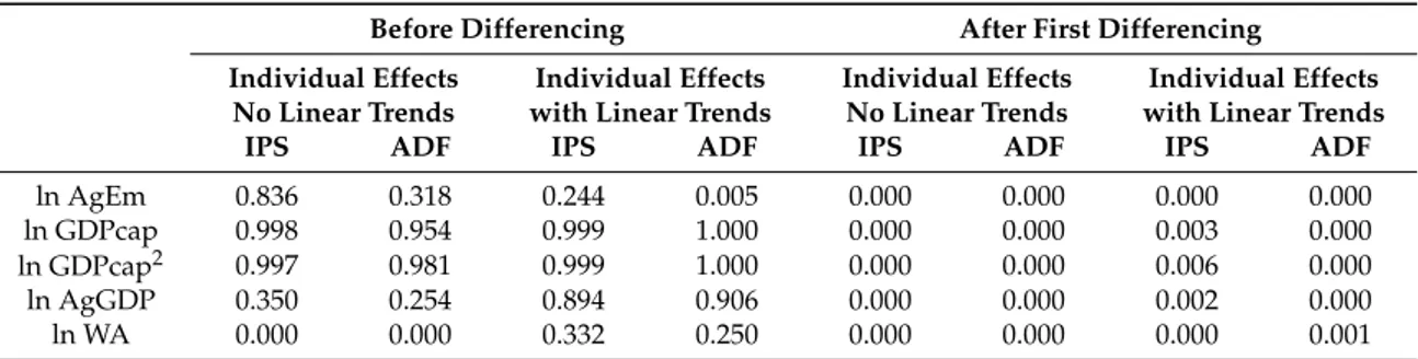
According to the unit root test results, for both the individual effect alone and the individual effect coupled with the linear trend, the null hypothesis of having unit root is not rejected neither by the IPS level analysis nor by the ADF tests. After first differencing, however, we reject the null hypothesis of unit root, suggesting both GDP per capita and agricultural share in GDP are integrated by order one, I(1). The results of the unit root tests are reported in Table1.
Table 1.Unit Root test results.
Before Differencing After First Differencing
Individual Effects Individual Effects Individual Effects Individual Effects No Linear Trends with Linear Trends No Linear Trends with Linear Trends
IPS ADF IPS ADF IPS ADF IPS ADF
ln AgEm 0.836 0.318 0.244 0.005 0.000 0.000 0.000 0.000 ln GDPcap 0.998 0.954 0.999 1.000 0.000 0.000 0.003 0.000 ln GDPcap2 0.997 0.981 0.999 1.000 0.000 0.000 0.006 0.000 ln AgGDP 0.350 0.254 0.894 0.906 0.000 0.000 0.002 0.000 ln WA 0.000 0.000 0.332 0.250 0.000 0.000 0.000 0.001
We use both the trace and max-eigenvalue tests to indicate the existence of cointegrating vectors for models (4) and (5). Table2reports the Johansen multivariate cointegration statistics. The results support the presence of two cointegrating equations at the one percent significance level for model (4), confirming the long-run relationship among agricultural emissions, economic growth, and agricultural share. Similar results occur for model (5), supporting the presence of three cointegrating equations at the one percent significance level, corroborating the long-run relationship among agricultural emissions, economic growth, agricultural shares, and anomalies.
Table 2.Johansen cointegration test results. NO. of Cointegrating
Equations
Model (4) Model (5)
Trace Statistics Max Eigenvalue Trace Statistics Max Eigenvalue
R = 0 168.22 * 113.34 * 300.13 * 139.53 *
R≤1 54.87 * 44.99 * 160.60 * 106.43 *
R≤2 9.89 6.87 54.17 * 45.19 *
R≤3 3.01 3.01 8.98 6.69
Sustainability 2017, 9, 1989 11 of 17
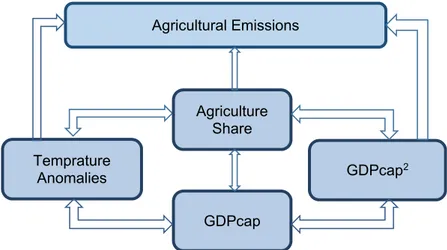
When looking at the direction of these relationships by running Granger causality tests, we see that almost all indicators cause each other, with the exception that while anomalies, squared GDP per capita, and agricultural shares are shown to cause agricultural emissions (resulting from nitrogen fertilizer), agricultural emissions do not appear to cause anomalies, squared GDP per capita, or agricultural shares. Figure7presents the direction of significant causalities in the long-run.
Sustainability 2017, 9, 1989 11 of 17
fertilizer), agricultural emissions do not appear to cause anomalies, squared GDP per capita, or agricultural shares. Figure 7 presents the direction of significant causalities in the long-run.
Figure 7. Causalities in the long-run.
After investigating the long-run dynamics among these variables and the direction of these relationships, we also checked the adjustment parameter ECT values that we obtained from the VECM results. ECT values measure the corresponding speed of adjustment in the variable with respect to the past deviation of the level variable from its equilibrium. We present the ECT results in the first row of Table 3. As seen from the t-statistics of ECT, the adjustment parameter is statistically significant, confirming that long-run causality among variables exists; the coefficient, however, is zero. In other words, disequilibrium in the agricultural emissions is not eliminated within a year. How long it would take for an adjustment from deviation towards the equilibrium is unclear. Therefore, we continue our analysis with short-run effects to understand the relationship between agricultural emissions and economic growth. Rows 2–5 in Table 3 below, presents the VECM results, that is, the short-run causal relationship among the variables of interest.
Table 3. VECM results—Short-run analysis. Dependent Var:
AgEm
Model (4) Model (5)
Coefficient t-Stat Prob Coefficient t-Stat Prob
ECT 0.001 5.05 0.000 0.000 3.88 0.000
GDPcap (−1) 0.598 2.12 0.034 0.904 3.36 0.001
GDPcap2 (−1) −0.034 −2.00 0.045 −0.051 −3.05 0.002
AgGDP (−1) 0.041 1.94 0.053 0.044 4.03 0.000
WA (−1) 0.011 4.07 0.000
According to the results agricultural emissions from nitrogen fertilizer use is caused by GDP per capita, suggesting first an increase in agricultural emissions as income increases, then a decrease in agricultural emissions after reaching a certain level of income. We control for agricultural shares when investigating the EKC. The results indicate a positive significant effect from agricultural shares. As expected, an increase in agricultural shares in GDP increases agricultural activities, and thus agricultural emissions.
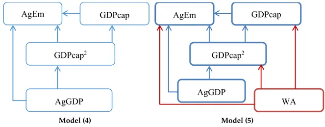
In the second model, when we add the anomaly indicator to the system, we see that the results do not change much, suggesting the stability of the model, like agricultural shares, anomalies are also significant and positive, suggesting that extreme temperatures have a positive effect on agricultural emissions. Figure 8 presents the directions of the short-run causalities. We also calculate the turning points of the agricultural emissions depending on the level of income. The turning point of the first model is calculated as 6595.33USD (exp (−0.5 (0.598/−0.034)), suggesting that after this level of GDP
Agricultural Emissions GDPcap GDPcap2 Agriculture Share Temprature Anomalies
Figure 7.Causalities in the long-run.
After investigating the long-run dynamics among these variables and the direction of these relationships, we also checked the adjustment parameter ECT values that we obtained from the VECM results. ECT values measure the corresponding speed of adjustment in the variable with respect to the past deviation of the level variable from its equilibrium. We present the ECT results in the first row of Table3. As seen from the t-statistics of ECT, the adjustment parameter is statistically significant, confirming that long-run causality among variables exists; the coefficient, however, is zero. In other words, disequilibrium in the agricultural emissions is not eliminated within a year. How long it would take for an adjustment from deviation towards the equilibrium is unclear. Therefore, we continue our analysis with short-run effects to understand the relationship between agricultural emissions and economic growth. Rows 2–5 in Table3below, presents the VECM results, that is, the short-run causal relationship among the variables of interest.
Table 3.VECM results—Short-run analysis.
Dependent Var: AgEm Model (4) Model (5)
Coefficient t-Stat Prob Coefficient t-Stat Prob
ECT 0.001 5.05 0.000 0.000 3.88 0.000
GDPcap (−1) 0.598 2.12 0.034 0.904 3.36 0.001 GDPcap2(−1) −0.034 −2.00 0.045 −0.051 −3.05 0.002 AgGDP (−1) 0.041 1.94 0.053 0.044 4.03 0.000
WA (−1) 0.011 4.07 0.000
According to the results agricultural emissions from nitrogen fertilizer use is caused by GDP per capita, suggesting first an increase in agricultural emissions as income increases, then a decrease in agricultural emissions after reaching a certain level of income. We control for agricultural shares when investigating the EKC. The results indicate a positive significant effect from agricultural shares. As expected, an increase in agricultural shares in GDP increases agricultural activities, and thus agricultural emissions.
Sustainability 2017, 9, 1989 12 of 17
In the second model, when we add the anomaly indicator to the system, we see that the results do not change much, suggesting the stability of the model, like agricultural shares, anomalies are also significant and positive, suggesting that extreme temperatures have a positive effect on agricultural emissions. Figure8presents the directions of the short-run causalities. We also calculate the turning points of the agricultural emissions depending on the level of income. The turning point of the first model is calculated as 6595.33USD (exp (−0.5 (0.598/−0.034)), suggesting that after this level of GDP per capita, agricultural emissions may start to decrease. As expected, the turning point is slightly higher for the second model, at 7,063.85 USD (exp (−0.5 (0.904/−0.051)).
Sustainability 2017, 9, 1989 12 of 17
per capita, agricultural emissions may start to decrease. As expected, the turning point is slightly higher for the second model, at 7,063.85 USD (exp (−0.5 (0.904/−0.051)).
Model (4) Model (5)
Figure 8. Short-run causalities. 4. Discussion and ConclusionS
To secure enough food for the growing world population, nitrogen fertilizers are indispensable inputs to crop production. As anthropogenic GHG emissions are responsible for climate change, the latter, in turn, has an impact on all natural systems, including humans. On one hand, agricultural activities cause environmental damage; on the other, they can play an important role in reversing environmental problems by the use of carbon sink, enhancing the infiltration of water, and preserving rural landscapes and biodiversity [39]. These positive effects can be achieved by using sustainable production methods. Therefore, researchers must understand the economic impact resulting from the human alteration of the nitrogen cycle.
It is important to study fully the link between climate change and the consumption of nitrogen fertilizer, which this study has done by econometrically analyzing panel data from 145 countries over a nine-year period from 2002 to 2010. The study captures economic and agricultural activities as well as agricultural emissions from these activities and temperature anomalies in this causal relationship. Both the long-run and the short-run relationships between these variables are studied. The results show that there is a statistically significant long-run causality among these variables. It is a unidirectional causality that runs from temperature anomalies, squared GDP per capita, and agricultural share to agricultural emissions resulting from nitrogen fertilizer. Agricultural emissions do not cause these variables. Although the results of the study show that agricultural emissions from the use of nitrogen fertilizers do not cause temperature anomalies, this does not mean that there is no feedback loop from agricultural emissions to climate.
The results also indicate that any disequilibrium taking place in agricultural emissions is not eliminated within a year. How long it would take for an adjustment from deviations towards equilibrium is unclear. Therefore, the results emphasize the challenge in managing agricultural emissions in the presence of temperature anomalies. The temperature anomalies are a main indicator of climate change [60,61,66]. Thus, agricultural practices under global climate change should involve not only technical solutions, but also adoptive approaches regarding the use of nitrogen fertilizer by farmers: responsive but cautious regulations of its use and economic schemes to stabilize the system. Farm-level adaptations, including changes in planting data, variety and crop, and applications of irrigation and fertilizer, are specifically presented in the literature in discussing the impact of global climate change on food supply [67,68]. The farmers’ efforts and activities might include, as suggested in studies by Scott [68]: soil and plant testing; minimized fallow periods; optimized split applications; and better fertilizer technology (such as nitrification inhibitors, time release, advanced delivery, advanced cultivars, and improved productivity of plants).
AgEm
GDPcap
GDPcap
2AgGDP
AgEm
GDPcap
GDPcap
2AgGDP
WA
Figure 8.Short-run causalities. 4. Discussion and Conclusions
To secure enough food for the growing world population, nitrogen fertilizers are indispensable inputs to crop production. As anthropogenic GHG emissions are responsible for climate change, the latter, in turn, has an impact on all natural systems, including humans. On one hand, agricultural activities cause environmental damage; on the other, they can play an important role in reversing environmental problems by the use of carbon sink, enhancing the infiltration of water, and preserving rural landscapes and biodiversity [39]. These positive effects can be achieved by using sustainable production methods. Therefore, researchers must understand the economic impact resulting from the human alteration of the nitrogen cycle.
It is important to study fully the link between climate change and the consumption of nitrogen fertilizer, which this study has done by econometrically analyzing panel data from 145 countries over a nine-year period from 2002 to 2010. The study captures economic and agricultural activities as well as agricultural emissions from these activities and temperature anomalies in this causal relationship. Both the long-run and the short-run relationships between these variables are studied. The results show that there is a statistically significant long-run causality among these variables. It is a unidirectional causality that runs from temperature anomalies, squared GDP per capita, and agricultural share to agricultural emissions resulting from nitrogen fertilizer. Agricultural emissions do not cause these variables. Although the results of the study show that agricultural emissions from the use of nitrogen fertilizers do not cause temperature anomalies, this does not mean that there is no feedback loop from agricultural emissions to climate.
The results also indicate that any disequilibrium taking place in agricultural emissions is not eliminated within a year. How long it would take for an adjustment from deviations towards equilibrium is unclear. Therefore, the results emphasize the challenge in managing agricultural emissions in the presence of temperature anomalies. The temperature anomalies are a main indicator of climate change [60,61,66]. Thus, agricultural practices under global climate change should involve not only technical solutions, but also adoptive approaches regarding the use of nitrogen fertilizer by
Sustainability 2017, 9, 1989 13 of 17
farmers: responsive but cautious regulations of its use and economic schemes to stabilize the system. Farm-level adaptations, including changes in planting data, variety and crop, and applications of irrigation and fertilizer, are specifically presented in the literature in discussing the impact of global climate change on food supply [67,68]. The farmers’ efforts and activities might include, as suggested in studies by Scott [68]: soil and plant testing; minimized fallow periods; optimized split applications; and better fertilizer technology (such as nitrification inhibitors, time release, advanced delivery, advanced cultivars, and improved productivity of plants).
Furthermore, as part of the policies or as an alternative approach to current agricultural practices, the premise of organic farming in curbing GHG emissions and in improving environmental quality and ecosystem services needs to be investigated. As eco-efficiency is certainly an important measure to be used in the mitigation of climate change in the agriculture sector, the promises of organic farming practices still need to be investigated in regard to their roles in climate-friendly agriculture. Skinner et al. [69] provide scientific evidence that concerning nitrous oxide emissions, there is a discrepancy observed between organically- and conventionally- managed soils. Their meta-analysis finds that the nitrous oxide emissions resulting from organically managed soils when scaled to the area of cultivated land are lower than when crop yield-scaled. The discrepancy is due to 26 percent less crop yield under organic management; thus, to equalize the nitrous oxide emissions per yield, there needs to be a 9 percent increase in crop yield in organic systems.
The results for the short-run lead us to a conclusion that as the incomes of countries increase, agricultural emissions decline. In a similar vein as has been shown in EKC studies [9], the effective use of nitrogen fertilizers as well as other associated agricultural practices can be achieved as countries reach a certain level of income per capita, approximately 7000 USD in this study. The similar results are obtained for 31 provincial economies in mainland China where the inverted U shaped EKC with a turning point of 10000–13000 CNY, for synthetic nitrogen indicator [7]. Management of externalities and environmental-friendly practices in agriculture requires resources that are possible within certain level of income. In addition, the results from the study indicate that when structures of economies shift to the agricultural sector, the use of nitrogen fertilizers, and thus emissions, also increases.
The results further indicate that temperature anomalies increase emissions from nitrogen fertilizers. This could be due to the fact that the potential negative effects of these anomalies are mitigated by farmers through changes in crop-production inputs (e.g., seeds, fertilizer, pesticides, and labor) as found in a Chinese field survey [8] and in the work by Mendelsohn [3]. As the global climate changes, temperature anomalies will be observed more frequently in certain parts of the world. This may lead to excessive and inefficient use of nitrogen fertilizers by farmers. Thus, economic, national, and global incentives should be aligned. To improve fertilizer use by farmers, economic incentives such as agricultural insurance can be introduced.
It is important to understand at the macro level what factors have been historically important in affecting emissions from nitrogen fertilizer use in the agricultural sector in the presence of temperature anomalies resulting from climate change. Temperature anomalies could result in great losses in the agricultural sector. This study aims to reveal some of the information available when reviewing historical data. However, this was done under data limitations, i.e., agricultural emission data was available only for nine years, which in turn limited the use of other climate indicators. Moreover, the other important variables at the regional and local level, the agronomic data such as soil temperature, soil moisture and clouds, were not available at the global level [9,58]. Aggregating the regional and local agronomic data at a global level, and also making them available on a global level, is in itself a large project requiring significant resources. Further, current FAO statistics do not include agronomic data on a global scale [44]. Creating such data would require collaboration across nations with intergovernmental agencies. Therefore, creating an aggregate agronomic data set is beyond the scope and aim of this study.
However, this study checks for the robustness of its results when such agronomic variables are missing. One example of this “check” is the use of arable land data, that is, temporary agricultural
Sustainability 2017, 9, 1989 14 of 17
crops, meadows, markets, kitchen gardens, and fallow. Arable land data can represent land use across countries at a more refined level. Some agronomic variables such as soil moisture and temperature can determine, at least implicitly, the allocation of land across different usages, and thus the size of arable land in countries. The models were run by including arable land variables in addition to the existing model variables. The actual data available is one of the challenging issues in this line of research. As more data becomes available, in future studies it will be possible to integrate agronomic data and climate indicators with economic data to study the interaction among the three.
There are other possible studies that could be conducted on regional, local and meso scales, by incorporating the drivers of nitrous oxide emissions based on agronomic characteristics such as crop and soil type, precipitation, and cropping systems. Much of the agronomic and social science literature incorporates these variables. Porter, J. R. et al. [52] state that as the field of climate detection and attribution advances to finer spatial and temporal scales, and as agricultural modeling studies expand to broader scales (from local and regional to global), there will be more opportunities for linking climate and crop studies. Therefore, this study adds a new piece to existing literature in its effort to analyze fertilizer use, economics growth, and agricultural emissions on a global level.
Acknowledgments:We thank for the two anonymous referees for their detailed and constructive comments. Author Contributions:Authors equally share the contributions. Both authors conceived the research problem, construct the models, and gathered data, and wrote the paper. Bahar Celikkol Erbas conducted the literature review and analyze the results. Ebru Guven Solakoglu conducted econometric analysis.
Conflicts of Interest:The authors declare no conflict of interest. References
1. Mendelsohn, R.; Dinar, A.; Williams, L. Distributional Impact on Climate Change on Rich and Poor Countries. Environ. Dev. 2006, 11, 159–178. [CrossRef]
2. Food and Agriculture Organization (FAO). Statistical Year Book 2012. World Food and Agriculture in Sustainability Dimensions, Climate Change. 2012. Available online: http://www.fao.org/docrep/015/ i2490e/i2490e00.htm(accessed on 10 February 2014).
3. Mendelsohn, R. The Impact of Climate Change on Agriculture in Developing Countries. J. Nat. Resour. Policy Res. 2009, 1, 5–19. [CrossRef]
4. Molua, E. An Empirical Assessment of the Impact of Climate Change on Smallholder Agriculture in Cameroon. Glob. Planet. Chang. 2009, 67, 205–208. [CrossRef]
5. Kabubo-Mariara, J.; Karanja, F.K. The economic impact of climate change on Kenyan crop agriculture: A ricardian approach. Glob. Planet. Chang. 2007, 57, 319–330. [CrossRef]
6. Zinyengere, N.; Crespo, O.; Hachigonta, S. Crop Response to Climate Change in Southern Africa: A Comprehensive Review. Glob. Planet. Chang. 2013, 111, 118–126. [CrossRef]
7. Chen, Y.; Wu, Z.; Okamoto, K.; Han, X.; Ma, G.; Chien, H.; Zhao, J. The Impacts of Climate Change on Crops in China: A Ricardian Analysis. Glob. Planet. Chang. 2013, 104, 61–74. [CrossRef]
8. Chen, H.; Wang, J.; Huang, J. Policy support, social capital, and farmers’ adaptation to drought in China. Glob. Environ. Chang. 2014, 24, 193–202. [CrossRef]
9. Zhang, X.; Davidson, E.A.; Mauzerall, D.L.; Searchinger, T.D.; Dumas, P.; Shen, Y. Managing Nitrogen for Sustainable Development. Nature 2015, 528, 51–59. [CrossRef] [PubMed]
10. Li, F.; Dong, S.; Li, F.; Yang, L. Is there an inverted U-shaped curve? Empirical analysis of the environmental Kuznets curve in agrochemicals. Front. Environ. Sci. Eng. 2016, 10, 276–287. [CrossRef]
11. Kijima, M.; Nishide, K.; Ohyama, A. Economic models for the environmental Kuznets Curve: A survey. J. Econ. Dyn. Control 2010, 34, 1187–1201. [CrossRef]
12. Stern, D.I. The rise and fall of environmental Kuznets Curve. World Dev. 2004, 32, 1419–1439. [CrossRef] 13. Grossman, G.M.; Krueger, A.B. Environmental Impact of a North American Free Trade Agreement; Working Paper
No. 3914; NBER: Cambridge, MA, USA, 1991.
Sustainability 2017, 9, 1989 15 of 17
15. Brock, W.A.; Taylor, M.S. Economic growth and the environment: A review of theory and empirics. In Handbook of Economic Growth; Aghion, P., Durlauf, S.N., Eds.; Elsevier: Amsterdam, The Netherlands, 2005; Volume 1B.
16. Grossman, G.M.; Krueger, A.B. Environmental Impact of a NAFTA. In The US—Mexico Free Trade Agreement; Garver, P.M., Ed.; MIT Press: Cambridge, MA, USA, 1993; pp. 13–56.
17. Selden, T.M.; Song, D. Environmental Quality and Development: Is there a Kuznets Curve for Air Pollution Emissions? J. Environ. Econ. Manag. 1994, 27, 147–162. [CrossRef]
18. Shafik, N.; Bandyopadhyay, S. Economic Growth and Environmental Quality: Time Series and Cross Section Evidence; World Bank: Washington, DC, USA, 1992.
19. Archibald, A.O.; Bochniarz, Z.; Gemma, M.; Srebotnjak, T. Transition and Sustainability: Empirical analysis of environmental Kuznets curve for water pollution in 25 countries in Central and Eastern Europe and the Commonwealth of Independent States. Environ. Policy Gov. 2009, 19, 73–98. [CrossRef]
20. Carson, R.T.; Jeon, Y.; McCubbin, D. The relationship between air pollution and emissions: US data. Environ. Dev. Econ. 1997, 2, 433–450. [CrossRef]
21. Carson, R.T. The Environmental Kuznets Curve: Seeking Empirical Regularity and Theoretical Structure. Rev. Environ. Econ. Policy 2010, 4, 3–23. [CrossRef]
22. Borghesi, S. The environmental Kuznets curve: A critical survey. In Economic Institutions and Environmental Policy, Ashgate; Franzini, M., Nicita, A., Eds.; Fondazione ENI Enrico Mattei: Milano, Italy, 2001.
23. Borghesi, S.; Vercelli, A. Sustainable globalization. Ecol. Econ. 2003, 44, 77–89. [CrossRef]
24. Grossman, G.M.; Krueger, A.B. Economic Growth and the Environment. Q. J. Econ. 1995, 110, 353–377. [CrossRef]
25. Magnani, E. The environmental Kuznets curve: Development path or policy results? Environ. Model. Softw. 2001, 16, 157–165. [CrossRef]
26. Stern, D.I.; Common, M.S.; Barbier, E.B. Economic growth and environmental degradation: The environmental Kuznets curve and sustainable development. World Dev. 1996, 24, 151–1160. [CrossRef] 27. Pearson, P.J. Energy, externalities and environmental quality: Will development cure the ills it creates?
Energy Stud. Rev. 1994, 6, 199–216. [CrossRef]
28. Frankel, J.A.; Rose, A.K. Is Trade Good or Bad for the Environment? Sorting Out the Causality; Working Paper 9201; National Bureau of Economic Research: Cambridge, MA, USA, 2002.
29. Vukina, T.; Beghin, J.C.; Solakoglu, E.G. Transition to Markets and the Environment: Effects of the Change in the Composition of Manufacturing Output. Environ. Dev. Econ. 1999, 4, 582–598. [CrossRef]
30. Solakoglu, E.G. The Effect of Property Rights on the Relationship between Economic Growth and Pollution for Transition Economies. East. Eur. Econ. 2007, 45, 77–94. [CrossRef]
31. Ang, J. CO2 emissions, energy consumption, and output in France. Energy Policy 2007, 35, 4772–4778. [CrossRef]
32. Apergis, N.; Ozturk, I. Testing Environmental Kuznets Curve hypothesis in Asian countries. Ecol. Indic. 2015, 52, 16–22. [CrossRef]
33. Wang, Y.; Kang, L.; Wu, X.; Xiao, Y. Estimating the environmental Kuznets curve for ecological footprint at the global level: A spatial econometric approach. Ecol. Indic. 2013, 34, 15–21. [CrossRef]
34. Al-muali, U.; Wend-Wai, C.; Sheau-Ting, L.; Mohammed, A.H. Investigating the Environmental Kuznets curve (EKC) hypothesis by utilizing the ecological footprint as an indicator of environmental degradation. Ecol. Indic. 2015, 48, 315–323. [CrossRef]
35. Wang, L.; Zhou, D.; Wang, Y.; Zha, D. An empirical study of the environmental Kuznets curve for environmental quality in Gansu province. Ecol. Indic. 2015, 56, 96–105. [CrossRef]
36. Tan, F.; Lean, H.; Khan, H. Growth and environmental quality in Singapore: Is there any trade-off? Ecol. Indic. 2015, 47, 149–155. [CrossRef]
37. Akbostancı, E.; Türüt-A¸sık, S.; Tunç, G.I. A decomposition analysis of CO2emissions from energy use: Turkish Case. Energy Policy 2009, 37, 4689–4699.
38. Leukhardt, F.; Allen, S. How environmentally focused is the German sustainability strategy? A critical discussion of the indicators used to measure sustainable development in Germany. Environ. Dev. Sustain. 2013, 15, 149–166. [CrossRef]
39. Erisman, J.W.; Galloway, J.; Seitzenger, S.; Bleeker, A.; Butterbach-Bahl, K. Reactive Nitrogen in the Environment and Its Effect on Climate Change. Curr. Opin. Environ. Sustain. 2011, 3, 281–290. [CrossRef]
Sustainability 2017, 9, 1989 16 of 17
40. Erisman, J.W.; Sutton, M.A.; Galloway, J.; Klimont, Z.; Winiwater, W. How a Century of Ammonia Synthesis Changed the World. Nat. Geosci. 2008, 1, 636–639. [CrossRef]
41. Chen, J.; Tang, C.; Sakura, Y.; Yu, J.; Fukushima, J. Nitrate Pollution from Agriculture in Different Hydrogeological Zones of the Regional Groundwater Flow System in the North China Plain. Hydrogeol. J. 2005, 13, 481–492. [CrossRef]
42. Galloway, J.N.; Townsend, A.R.; Erisman, J.W.; Bekunda, M.; Cai, Z.; Freney, J.R.; Martinelli, L.A.; Seitzinger, S.P.; Sutton, M.A. Transformation of the Nitrogen Cycle, Recent Trends, Questions, and Potential Solutions. Science 2008, 320, 889–892. [CrossRef] [PubMed]
43. Vitousek, P.M.; Aber, C.D.; Howarth, R.W.; Likens, G.E.; Matson, P.A.; Schindler, D.W.; Schlesinger, W.H.; Tilman, D.G. Human Alterations of the Global Nitrogen Cycyle: Sources and Consequences. Ecol. Appl. 1997, 7, 737–750.
44. Food and Agriculture Organization of the United Nations (FAOSTAT). Available online:http://www.fao. org/faostat/en/#data/RA(accessed on 21 July 2017).
45. WDI, World Development Indicators. Available online:http://databank.worldbank.org/data/reports.aspx? source=world-development-indicators(accessed on 21 July 2017).
46. Gellings, C.W.; Parmenter, K.E. Energy Efficiency in Fertilizer Production and Use. In Efficienct Use and Conservation Energy; Gellings, C.W., Blok, K., Eds.; Encyclopedia of Life Support Systems (EOLSS), Eolss Publishers: Oxford, UK, 2004.
47. Food and Agriculture Organization (FAO). Compendium of Agricultural-Environmental Indicators 1989–1991 to 2000; FAO of UN: Rome, Italy, 2003.
48. Intergovernmental Panel on Climate Change (IPCC) (WGII). Climate Change 2001: Impacts, Adaptation, and Vulnerability. Contribution of Working Group II to the Third Assessment Report of the Intergovernmental Panel on Climate Change; McCarthy, J.J., Canziani, O.F., Leary, N.A., Dokken, D.J., White, K.S., Eds.; Cambridge University Press: Cambridge, UK, 2001.
49. Intergovernmental Panel on Climate Change (IPCC). Climate Change 2007: The Physical Science Basis; Cambridge University Press: Cambridge, UK, 2007.
50. Rosenzweig, C.; Parry, M.L. Potential Impact of Climate Change on World Food Supply. Nature 1994, 367, 133–138. [CrossRef]
51. Rosenzweig, C.; Hillel, D. Climate Change and the Global Harvest: Potential Impacts of the Greenhouse Effect on Agriculture; Oxford University Press: New York, NY, USA, 1998; p. 324.
52. Porter, J.R.; Xie, A.J.L.; Challinor, K.A.J.; Cochrane, S.M.K.; Howden, MS.M.; Iqbal, D.B.M.M.; Lobell, D.B.; Travasso, M.I. Food security and food production systems. In Climate Change 2014: Impacts, Adaptation, and Vulnerability. Part A: Global and Sectoral Aspects; Field, C.B., Barros, V.R., Dokken, D.J., Mach, K.J., Mastrandrea, M.D., Bilir, T.E., Chatterjee, M., Ebi, K.L., Estrada, Y.O., Genova, R.C., et al., Eds.; Cambridge University Press: Cambridge, UK, 2014; pp. 485–533.
53. Peng, S.; Huang, J.; Sheehy, J.E.; Laza, R.C.; Visperas, R.M.; Zhong, X.; Centeno, G.S.; Khush, G.S.; Cassman, K.G. Rice yields decline with higher night temperature from global warming. Proc. Natl. Acad. Sci. USA 2004, 101, 9971–9975. [CrossRef] [PubMed]
54. Wassmann, R.; Jagadish, S.V.K.; Heur, S.; Ismail, A.; Redona, E.; Serraj, R.; Singh, R.K.; Howell, H.; Pathak, G.; Sumfleth, K. Climate change affecting rice production: The physiological and agronomic basis for possible adaptation strategies. In Advances in Agronomy; Sparks, D.L., Ed.; Elsevier Science: Amsterdam, The Netherlands, 2009; Volume 101.
55. Welch, J.R.; Vincent, J.R.; Auffhammer, M.; Moya, P.F.; Dobermann, A.; Dawe, D. Rice yields in tropical/subtropical Asia exhibit large but opposing sensitivities to minimum and maximum temperatures. Proc. Natl. Acad. Sci. USA 2010, 107, 14562–14567. [CrossRef] [PubMed]
56. Porter, J.R.; Gawith, M. Temperatures and the growth and development of wheat: A review. Eur. J. Agron. 1999, 10, 23–36. [CrossRef]
57. Schlenker, W.; Roberts, M.J. Nonlinear temperature effects indicate severe damages to U.S. crop yields under climate change. Proc. Natl. Acad. Sci. USA 2009, 106, 15594–15598. [CrossRef] [PubMed]
58. Christidis, N.; Stott, P.A.; Brown, S.; Hegerl, G.C.; Caesar, J. Detection of changes in temperature extremes during the second half of the 20th century. Geophys. Res. Lett. 2005. [CrossRef]
59. Zwiers, F.W.; Zhang, X.; Feng, Y. Anthropogenic influence on long return period daily temperature extremes at regional scales. J. Clim. 2011, 24, 881–892. [CrossRef]
Sustainability 2017, 9, 1989 17 of 17
60. Goddard Institute for Space Studies’ (GISS), National Aeronautics and Space Administration (NASA). Available online: http://data.giss.nasa.gov/gistemp/tabledata_v3/ZonAnn.Ts+dSST.txt (accessed on 23 January 2014).
61. National Oceanic and Atmospheric Administration, National Climatic Data Center, Global Surface Temperature Anomalies. Available online: https://www.ncdc.noaa.gov/monitoring-references/faq/ anomalies.php(accessed on 4 June 2014).
62. Cole, M.A.; Rayner, A.; Bates, J.M. The Environmental Kuznets Curve: An empirical analysis. Environ. Dev. Econ. 2001, 2, 401–416. [CrossRef]
63. Dickey, D.A.; Fuller, W.A. Likelihood Ratio Statistics for Autoregressive Time Series with a Unit Root. Econometrica 1981, 49, 1057–1072. [CrossRef]
64. Im, K.S.; Pesaran, M.H.; Shin, Y. Testing for Unit Roots in Heterogeneous Panels. J. Econom. 2003, 115, 53–74. [CrossRef]
65. Johansen, S.; Juselius, K. Testing Structural Hypotheses in a Multivariate Cointegration Analysis of the PPP and the UIP for UK. J. Econ. 1992, 53, 211–244. [CrossRef]
66. NASA. A blanket around the Earth. Available online: http://climate.nasa.gov/causes (accessed on 8 February 2014).
67. Schneph, R. Energy Use in Agriculture: Background and Issues. Available online: http:// nationalaglawcenter.org/wp-content/uploads/assets/crs/RL32677.pdf(accessed on 25 October 2017). 68. Scott, M.J.; Sands, R.D.; Rosenberg, N.J.; Izaurralde, R.C. Future N2O from US Agriculture: Projecting Effects
of Changing Land Use, Agricultural Technology and Climate on CO2emissions. Glob. Environ. Chang. 2002, 12, 105–115. [CrossRef]
69. Skinner, C.; Gattinger, A.; Muller, A.; Mader, P.; FlieBbach, A.; Stolze, M.; Ruser, R.; Niggli, U. Greenhouse Gas Fluxes from Agricultural Soils under Organic and Non Organic Management—A Global Meta-Analysis. Sci. Total Environ. 2014, 468–469, 553–563. [CrossRef] [PubMed]
© 2017 by the authors. Licensee MDPI, Basel, Switzerland. This article is an open access article distributed under the terms and conditions of the Creative Commons Attribution (CC BY) license (http://creativecommons.org/licenses/by/4.0/).