On the stabilization of the wave equation

O n t h e S t a b i l i z a t i o n o f t h e W a v e E q u a t i o n

()met Morgfil

Bilkent University, Dept. of Electrical and Electronics Engineering 06533, Bilkent, Ankara, Turkey

c-mall : morgul@trbilun.bitnet

1

I n t r o d u c t i o n

Many mechanical systems, such as spacecraft with flexible attachements, or robots with flexible links, and many practical systems such as power systems, mass transport systems contain certain parts whose dynamic behaviour can be rigorously described only by partial differential equations (PDE). In such systems, to achieve high precision demands, the dynamic effect of the system parts whose behaviour are described by PDE's on the overall system has to be taken into account in designing the controllers.

In recent years, boundary control of systems represented by PDE's has become an important research area. This idea is first applied to the systems represented by the wave equation (e.g. elastic strings, cables), [2], [18], [9], and recently extended to the beam equations, [3], and to the rotating flexible structures, [12]. In particular, it has been shown that for a string which is clamped at one end and is free at the other end, a single

non-dynamic

boundary control applied at the free end is sufficient to exponentially stabilize the system, [2]. A good source of references to papers in which boundary stabilization problems are treated can be found in [1%

In this note, we consider a linear time invariant system which is represented by one-dimensional wave equation in a bounded domain. We assume that the system is clamped at one end and the boundary control input is applied at the other end. For this system, we propose a finite dimensional

dynamic

boundary controller. The transfer function of the controller is restricted to be a strictly positive real function. (We note that this class of controllers has been applied to the stabilization of the Euler-Bernoulli beam equation, see [13]).

This

class of controllers is quite large and contains some previously proposed

non-dynamic

controllers as a special case. We show that, if the controller transfer function is strictly proper, the resulting closed-loop system is

asyraptotically,

but not

exponentially

stable. The main advantage of this type of controller is that the resulting open-loop map is also strictly proper, which is important in proving certain stability robustness results, see [6]. On the oflmr hand, if the controller transfer hmction is proper but not strictly proper, we show that the resulting closed-loop system is

ezponenlially

stable.

This paper is organized as follows. In the next section we state the stabilization problem. In the section 3, we give the main stabilization results. Then, in the section 4 we pre~ent some numerical simulation results, which show the effect of the proposed stabilizing controller on the eigenvalues of the system. Then we give some concluding remarks.

532 2 P r o b l e m S t a t e m e n t

We consider a string as an example of a system whose behaviour is modeled by wave equation. Without loss of generality, we assume that the string length, mass density and the string tension are as L = l , p = 1 and T = 1, respectively. We denote the displacement of the string by y(:~,t) at z E (0,1) and t ~ 0. Futhermore, we assume that the string is fixed at one end and stabilized by

dynamic

boundary control at the other end. Thus the system under consideration is :

yu(z, t) = y==(z, t) x E C 0,1) t 2> 0 (1)

y(o,t) = o y.(1,t) =

-fi0

t >_

o (2)

where a subscript, as in Yl denotes a partial differential with respect to the corresponding variable, and f(-) : R+ --, t t is the boundary control force applied at the free end of the string. We note that the systems represented by (1), (2) are not restricted to strings; for example vibrations of long cables, the longitudinal motion and the torsional vibrations of elastic beams can also be represented

by these equations, see [I I]. W e assume that f(t) is generated by the following dynamic controller

w(1) = Am(t) + ~,(I, t) t >_ 0 (3)

f(t) = cTw(t) + dvl(l, t) t _> 0 (4)

where to E R " , for some natural number n, is tile actuator state, A E R "x" is a constant matrix, b, c E R ~ are constant column vectors, d is a constant real number and the superscript T denotes transpose. In case of a

non-dynamic

actuator, (3) will not exist, and (4) will reduce to

f(~) = dy,(1, g) t 2> 0 (5)

which is a case considered by [2]. Therefore, the actuator proposed above may be considered as a generalization of the control law given by (5), see [2], [181, [9]. Q

It is known that if the boundary control force is set to zero ( i.e. / - 0), then the system given by (1)-(2) has infinitely many eigenvalues on the imaginary axis, see e.g. [11]. Our problem is to design an actuator given by (3)-(4) such that the resulting system given by (1)-(4) is stable in some sense.

The stabilization problem stated above can be solved by means of a

non-dynamic

actuator. For example, in [2], it was proven that the system given by (1)-(2) and (5) is exponentially stable provided that d > 0. However, it was shown in [5] that the stability of this system is not robust with respect to arbitrarily small delays in the feedback loop. Moreover, the controller transfer function given by (5) is not strictly proper, which might cause some problems in actual implementation, see [6]. While we do not directly address these issues, the above discussion shows that in order to solve a variety of control problems, control laws more general than (5) are required. The main motivation of this paper is to propose a large class of finite dimensional stabilizing controllers for the system given by (1)-(2). The proposed

dynamic

controller given by (3)-(4) is a candidate for such a class which also covers the controller given by (5).

We also note that the proposed controller offers extra degree of freedom in designing the con- trollers. This extra degree of freedom could be exploited to solve a variety of control problems, such as

eigenvalue assignment, disturbance rejection, etc., while malnt~ning stability, see [17]. Preliminary simulation studies show that by using the controller given by (3)-(4), it could be possible to change the eigenvalues of the system given by (1)-(4) over a specified frequency range, without affecting the rest of the spectrum very much, (see the section 4). We note that this could not be achieved by using the controller given by (5), since in this case the spectrum of the system is affected uniformly.

3

Stability

Results

W e first m a k e the following assumptions thoroughout this work :

A s s u m p t i o n 1 : All eigenvMues of A G R ~x~ have negative real parts. A s s u m p t i o n 2 : ( A, b) is controllable and (c, A) is observable.

A s s u m p t i o n 3 : d > 0; moreover there exists a constant 7, d _> 7 -> 0, such that the following holds :

d + T~e{cr(jwl

-- A)-'b}

> 7, , w e R rq. (6) If we take the Laplace transform in (4) and (5) and use zero initial conditions, w e obtain :

](~) = [d + c r ( s ! - A)-Xb]~t(1, s) = g(5)•,(l, ~) (Z) where a hat denotes the Laplace transform of the corresponding variable. This, together with (6) implies that the transfer function in (7) is a strictly positive real function, see [19].

Let the assumptions 1-3 stated above hold. Then, it follows from the Meyer-Kalman-Yakubovlcb Lemma, [19, p.133], that given any symmetric positive definite matrix Q E R " x ' , there exists a symmetric positive definite matrix P E R "x'~, a vector q E R ~ and a constant ~ > 0 satisfying :

AT p + PA = _qqr _ eQ (8)

e b - c = ~ q

(9)

To analyze the system given by (1)-(4), we first define the following function spaces :

n := {(u v w )r[u e H~,v e L2,w E R"} (10)

= {f: [0, L] --,

RlfoLf2dx

< co} (11)

L 2

H i = {f e L21f,

f',f",...

,f(~} e L 2, f(0) = 0} (12) The equations (I)-(4), can be written in the following abstr~t form :

= Lz , z(0) e ~ (13)

where z = (y yt w )~r E 7-/, the operator L : 7"/--~ 7"/is a linear unbounded operator defined as

L v = u.. (14)

534

The domain D(L) of the operator L is defined as :

DCL) := ((u v w )Tin E I ~ , v 6 H1o, to E K~; (15) uffi(l) + cxw + dr(l) = 0}

Let the assumptions 1-3 hold, let Q E R "x" be an arbitrary symmetric positive definite matrix and let P E R nxn, q E K ~ be the solutions of (8) and (9) where P is also a symmetric and positive definite matrix. In ~ , we define the following "energy" inner-product:

I t 1 t I T

(161

where z -- (y yt to )T, ~ ---- (~ Yt t~ )T. We note that 7-(, together with the energy inner-product given by (16) becomes a Hilbert space, [2]. The "energy" norm induced by (16) is :

1 l w T p t o (17)

E(0 := ;lz(t)ll~: -- ~ Jo' y,~d= + 1 f' 2 ~

_{i joy.}

₊

In the sequel we need the following inequality which follows from Jensen's inequality, [15, p.110]

Y2(=) -< K (y')~d~

W e (0,1)

Vy e H~

(16)

L e m m a 1 : Consider the system given by (1)-(4). Let the assumptions 1-3 hold. Then the energy E(t) given by (17) is a nonincreasing function of time along the classical solutions of (1)-(4). (For the terminology of partial differential equations and semigroup theory, the reader is referred to e.g. {14]).

P r o o f : By differentiating (17) with respect to time, using (1)-(4), integrating by parts and using (8)-(9), we obtain :

~* = fl o ytyudz Jr f~ yzyz, dz Jr 1(~TpW + toTp.~) (19)

= --~y~(1, t) - ½[Vf~d - 7)y,(1, t) -

t o T q ] 2 - -

~toTQto

where to obtain the first equation, we differentiated (17) with respect to time, to obtain the second equation we used (1)-(3), integration by parts, (4),(8), and finally (9).

Since E < 0, it follows that E(t) is a nonincreasing function of time along the classical solutions of (1)-(4). That is, we have

IIz(t)llg

< II*(O)llg, hence the system given by (1)-(4) is stable. Cl

T h e o r e m 1 : Consider the system given by (13), where the operator L is given by (14). Then i : The operator L generates a Co-semigroup T(t) on 7/,

ii : the Co-semigroup Tit ) generated by L is asymptotically stable, that is the energy given by (17) asymptotically tends to zero along the classical solutions of (13).

P r o o f :

i : We use Lumer-Phillips theorem, see [14, p.14]. From the [,emma 1 it follows that the operator L is dissipative on ?t, see (19). Hence, to prove the assertion i, it is enough to show that for some A > 0, the operator A I - A : 74 ---, ~ is onto. Let ( f h r ) T E X b e g i v e n . W e h a v e to find

(u v to )r E D(L) such that for some A > 0 :

Au - v = f , Av - u== = h (20)

~(0) = 0 ~,=(1) + cry, + dI~(1) = 0 (22) Using (20), we o b t a i n :

12u - u==

= h + Af (23)

whose solution satisfying u(0) = 0 is given by :

1

fo=(h(s) +

Af(s)) sinh A(z - s)ds z E (0,1)

u(x)

= cl sinh Ax - ~' (24)

where sinh(.) is the hyperbolic sine function. T h e constant cl can be uniquely d e t e r m i n e d from (22). T h e remaining u n k n o w n s v and w can be found from (20) and (21), respectively. It can easily be shown t h a t

(u v w )r E D(L).

This proves t h a t for all I > 0, the operator 1 / - A : 7"/--* is onto. Since 7"f is a Hilhert space, it follows t h a t

D(L)

is dense in 7"f, see [14, p.16]. Hence, by Lumer-Phillips theorem, it follows t h a t L generates a Co-semigroup

T(t)

on ~ .

ii : To prove the assertion ii, we use LaSalle's invariance principle, extended to infinite dimensional systems, see [16, p.78]. According to this principle, all solutions of (13) asymptotically tend to the maximal invariant subset of the following set :

S = {z E ~1 ~ = 0} (25)

provided t h a t the solutions are

precompact

in 7-/. T h e precompactness of the solutions are guaranteed if the operator 1 I - L : 9/ ---} ~ is compact for some A > 0. To prove the last property, we first show t h a t L ~x exists and is a compact operator on 7-L To see this, we put 1 = 0 in (20)-(22), which results in the following solution (u v w ) r E ~ for any given ( f h r ) r E 7"f z E ( 0, I) :

fZ'

where the constant c2 can be determined from (22). It follows t h a t 1;-1 exists and m a p s 7-/into Hg x I-I~ x R " , hence is a compact operator. This also proves t h a t the s p e c t r u m of L consists entirely of isolated eigenvMues, and t h a t for any I in the resolvent set of L, the operator ( 1 / - L) -1 : 7~ ~ ~ is a compact operator, see [8, p.187]. Furthermore, our argument above shows t h a t I = 0 is not an eigenvalue of L. This proves t h a t the solutions of (13) are precompact in ~ , hence by LaSalle's invariance principle, the solutions asymptotically tend to the m a x i m a l invariant subset of 6" (see (25)).

It can easily be shown t h a t the only classical solution of (13) which lies in S is the zero solution. To see this, we set /~ = 0 in (19), which results in w = 0. This implies t h a t tb = 0, hence by using (2)-(4) we o b t a i n V=(1, ~) = 0, y~(1, t) = 0. Since all boundary conditions are separable, the solution of (1) can be found by using separation of variables. T h a t is, the solution of (1)-(2) with the boundary conditions stated above assumes the form *d(z, t) =

A(t)B(z)

where the functions A : R + ---} R and B : [0, 1] ---} R are twice differentiable functions to be determined from t h e b o u n d a r y conditions. By using (1)-(2) and the b o u n d a r y conditions s t a t e d above, it can easily be shown t h a t either A -- 0, or B = 0, hence V(z, t) = 0. Hence, by La..qalle's invariance principle, we conlude t h a t the solutions of (13) asymptotically t e n d to the zero solution. Cl

R e m a r k 1 : Let us investigate the system given by (I)-(4) from an i n p u t / o u t p u t point of view. Let us define the b o u n d a r y control force f ( t ) as the input a n d / / t ( l ~ t ) as the output. If we take the Laplace transform of (1), use zero initial conditions, and use the b o u n d a r y conditions (2), we obtain

5 3 6

the plant transfer function p(s) as p(s) = - s l n h s/cosh s. Let C denote the set of complex numbers, and for ~ • 1t let C.+ = {s • C]~es _> ~}. Although p(s) is not bounded on the imaginary axis, it is bounded on C,+ for any ~ > 0, hence

proper

in this sense, (p • .4_(oo) with the notation of {6], see also [1]). Let us take d = 0 in the controller given by (4), which results in a strictly

proper

compansator g(8), see (7). The resulting open-loop map g(s)p(~) is also

strictly proper

in the sense that for any # > 0,

g(s)p(a)

-* 0 as I s I ~ oo, 8 E Ca+, see [6]. Hence, for the system given by (1)-(2), there exist

strictly proper

controllers for which the open-loop map is also strictly proper and the closed-loop system is stable in

asyraptotical

sense. However, if the stability is understood in

ezponential

sense, following [6], it can be shown that for the system given by (1)-(2) such a controller does not exist. This shows that for infinite dimensional systems, exponential stability requirement may be too restrictive, and that asymptotic stability requirement may be more suitable for designing controllers. This point requires further research, c3

The above argument shows that when d = 0, that is the controller given by (7) is

strictly proper,

the resulting closed-loop system cannot be exponentially stable. In the following we prove that if the controller is

proper

but not strictly proper, ( i.e. d > 0), exponential stability may be obtained. To prove this result, we use the following theorem which is due to Huang, [7] :

T h e o r e m 2 : [4], [7] Let T(t) be a C0-semigroup generated by a linear operator L in a Hilbert space. Assume that T ( 0 satisfies :

HT(t){{ < B t >_ 0 (27)

for some B > 0. Then, there exist M > 0 and 5 > 0 such that :

{IT(t){{ < M e -6' t > 0 (28)

if and only if the imaginary axis belongs to the resolvent set of L, and

sup l i ( j ~ l - L)-'I1 < o o o (29)

,#ER

For all application of this theorem to flexible structures, see [4].

T h e o r e m 3 : Consider the system given by (13). Assume that in the controller given by (3)-(4) we have d > 0; moreover there exists a constant ")' > 0 such that d _~ 7 and (6) is satisfied. (cf. with the assumption 3). Then the semigroup T(t) generated by the operator L given by (14) is exponentially stable.

R e m a r k 2 : The main distinction between the Theorem 3 and the Theorem 1 is that, in the Theorem 1, the real part of the transfer function,

7Ze(jw)

is required to be strictly positive, whereas ill the Theorem 3, it is required to be

bounded away

from zero. For the non-dynamic case, i.e. when tile controller is given by (5) with d > 0, instead of (3)-(4), the exponential stability was proven in I2]. Hence, tile result presented here may be considered as a generalization of that result. However, we note that the techniques we use in the following proof are entirely different than those employed in [2]. We also note that if (4) is replaced by

f(t) =cTw-bdy,(1,t)-bky(1,t)

P r o o f : By the Theorem 1, the operator L generates a Co-semigroup T(t) on 74. By the Lemma 1, this semigroup is hounded, i.e. (27) is satisfied. Also, by the Theorem 1, the spectrum of L consists entirely of countably many isolated eigenvalues, and )t = 0 is not an eigenvalue of L.

Next we prove by contradiction that the imaginary axis belongs to the resolvent set of L. Suppose that tile spectrum of L and the imaginary axis have common points. Since the operator L has point (i.e. discrete) spectrum, it follows that there exists a w E R such that (20)-(22) has a nontrivial solutions for )t = j w and ( f h r )T = (0 0 0 )r. These solutions are given as :

u(z) = c3sinwx v(z) = jwcssinwx w = c3jwsinto(fioI - A)-Xb z G (0,1) (30) where c3 is an arbitrary constant. Using (30) in (22) yields :

c3[wco$w + jw(cT(jwI -- A)~tb + d)sinw] = 0 (31) We define g(jw) as : g(jw) :-- R(w) + j l ( w ) where R(w) and l(w) are the real and imaginary parts of g(jw), respectively (see (7)). Using this in (31), we conclude that either cs = 0, or the following holds :

wcosw - w I ( w ) s i n w = 0 wR(w)sinw = 0 (32) Since ~ = 0 is not an eigenvalue of L, and since

R(w)

> q' > 0, Vw E R , it can easily be shown that (32) does not have any solution. Therefore, in (31) we must have e3 = 0, which, by (30) will yield to tile trivial solution. This shows that the imaginary axis does not belong to the spectrum of L, hence must belong to the resolvent of L, (note that L has point spectrum).

To prove the estimate (29), we first solve (20)-(22) for given ( f h r )r E 7"/and A = jw, w E R. By (24), the solution u which satisfies u(0) = 0 is given as :

u(x) = jclsinw~ - 1 fo=(h(s) + j w f ( s ) ) s i n w ( z - $)ds x e (0,1) (33) where

cl = f:(h(s) + jwf(s))(cosw(1 - s) + jg(jw)siraz(1 - s))ds -- c r ( j w l -- A ) - l r (34)

jwcosw -- wg(jw)sinw v(x) and w can he found from (20) and (21) as :

- j fo = (h(s) + jwf(s))sirua(z - s ) ~ - f ( z ) x e (0,1)

(35)

w = (jwI - A) -I [jwu(1)b + r I (36) By differentiating (33) with respect to x, using integration by parts, and (18), we obtain :

fo u'dx < 2w'c~ + IQ( fo' h2(z)ds + fo' (f')'(s)ds) (37) for some K~ > 0. Similarly, by using integration by parts and (18) in (35), we obtain :

for some 1i2 > 0. Also, by using (36), (18) and (37), we obtain :

5 3 8

To obtain a bound on we1 for large w, we consider the denominator of (34) :

n ( ~ ) ' =1 J cos ~ - a c i d ) sin ~ I'_> 7 ' sin' w + cos' ~ - 2 1 ( ~ ) sin ~ cos ~ (40)

where I " ] denotes the absolute value of a complex number. Since l(w) decays at least as O(1/w) for large ta, (see (7)), and since sin2w + cos2w = 1, it follows from (40) that there exists a constant Ks > 0 such that for oJ sufficiently large, we have D(w) > K3. Using this result and integration by parts in (34), we obtain the following estimate for large w :

!

+ ]0] (/')2 (~)d~ + llrll 2 +

(o,c,)' = g , ( ] ° h~(~)d~

f'(1)) (41)

for some/('4 > O.

Since II(jcal - A)-'II decays at least as 0(-~) for large w, by using (18), a~ad (37)-(41), we obtain tile following estimate for large w :

l 2

fo u=dx+ f o l V a d x + u 2 ( 1 ) + w r P w < ~ K ( f o I - h2(a)da + fo ( f ) (s)ds + 1 2

Ilrll")

(42)

for some K > 0.

Since the imaginary axis belongs to the resolvent set p(L) of the operator L, and since for each

A E p(L), (AI - L) -~ is compact, it follows that for any ft < oo,

sup

I I ( j w l - A)-111 < ~ (43)

Hence, from (42)-(43), we conclude that the estimate given by (29) holds. Therefore, by the Theorem 2, wc conclude that the Co-semigroup T(t) generated by the operator L is exponentially stable, that is (28) holds . O

4

N u m e r i c a l

R e s u l t s

Ill this section, to show the effect of tile proposed controller given by (3)-(4) on the eigenvalues of tile system given by (1)-(2), we present some numerical simulation results. By taking the Laplace transform, using (1)-(4), it can easily bc shown that the eigenvalues of the system given by (1)-(4) are the roots of the following equation :

cosh s + g(s) sinh s = 0 s E C C44)

where g(s) is given by (7). When g(s) ~ 0, (i.e uncontrolled system), the roots ,~ of (44) are all on the imaginary axis and are given by ,~ = jean, w~ = (2n - 1)1r/2, r~ = 1,2, ....

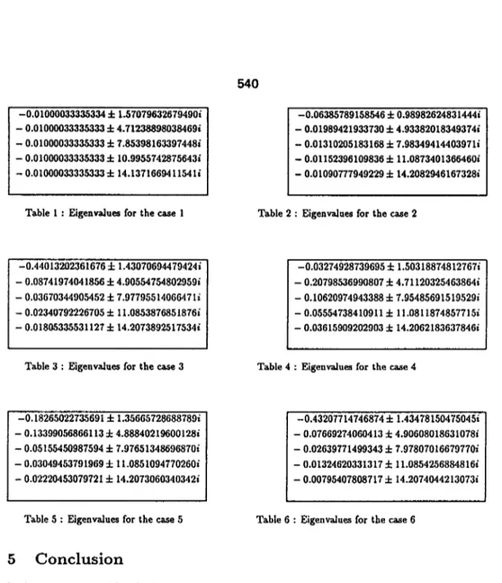
To see the difference between the effects of the non-dynamic and dynamic boundary control on the eigenvalues, we first consider the non-dynamic boundary control given by (5) with the following parameter :

case 1 : d = 0.0t

The first five roots of (44), listed with increasing imaginary parts, are shown in the Table 1. As call be seen, the roots are uniformly bounded away from the imaginary axis, and the imaginary parts are close to the imaginary parts of the roots of the uncontrolled system given above.

For some control applications it may be desirable to change the spectrum only over a prescribed frequency range. For example, t h e b e a m may be subject to a disturbance with a known frequency context. In this case, to reduce t h e effect of t h e disturbance, it m a y be desirable to introduce more d a m p i n g only to t h e m o d e s of t h e beam over t h e frequency range of the disturbance. Note t h a t this could be achieved by increasing d, but in that case the remaining modes are also affected uniformly, and t h e required actuator energy will possibly increase, which m a y cause saturation in t h e controller. To introduce more d a m p i n g only to the lower modes, we propose the following controller transfer function :

g ( s ) = d +

where, K , ~ and Wo are positive constants. T h e real part of g ( j w ) is given by :

K s

s~ +

2~os

+ ~o 2 (45)

TC.e{g(jw) } = d + 2K4w°w2 (46)

hence (6) is satisfied with q~ = d. T h e m a x i m u m of 7"¢.e{g(j~a)} is obtained at w --- wo and is given by :

K

m a x n e { g ( j w ) } - d + (47)

~,E R ~ 0

and 7?.e{g(j~a)} decreases to d as w --* 0 and as ~a ~ oo. Also note that the proposed dynamic controller does not increase uniformly t h e m i n i m u m of 7¢.e{g(jw)}, that is :

inf g e { g ( j ~ ) } = d (48)

taEIL

Since we want to decrease 7¢.e{Al} and Tq.e{A2}, where ,~l and ,~2 are first and second eigenvalues in tile Table 1, respectively, from t h e reasoning above we conclude that a good choice for this purpose is wo = Zm{)~l} or woi = Z m ( A ~ } We calculated the roots of (44) for the following choices of the controller parameters : case $ : d = 0.01, K = 1, ~ = 0.05, wo = ~r/2, case 3 : d = 0.01, K = 1, ~ = 0.5, wo = 7r/2, case 4 : d = 0.01, K = 1, ~ = 0.5, w0 = 37r/2, case 5 : d = 0.01, K = 1, ~ = 0.5, wo ---- 0.757r, case 6 : d = 0, K = 1, ~ = 0.5, wo = re/2,

In all cases, the first five roots of (44) are given in the Tables I-6. We note that these roots satisfy (44) with an error less than I0 - s . As it can be seen from the Tables 2-5, t h e resonant frequency wo of the controller transfer function determines the frequency (i.e. imaginary part) of the roots which are most affected. Table 6 Mso shows that in case t h e controller transfer function is strictly proper (i.e. d = 0), the real parts of the roots are still negative, b u t not uniformly bounded away from the imaginary axis. T h e calculations show that in this case, the real parts of 100th, 200th, and 500th roots are - 0 . 1 6 x 10 -4, - 0 . 3 9 x 10 - s , and - 1 . 5 5 x 10 -6, respectively.

-0.01000033335334 4- 1.57079632679490i - 0.01000033335333 4- 4.71238898038469i - 0.0100003333.5333 4- 7.85398163397448i - 0.01000033335333 4- 10.9955742875643i - 0.010000333353334- 14.1371669411541i

540

-0.06385789158546 4- 0.98982624831444i -0.019894219337304-4.93382018349374i - 0.013102051831684-7.98349414403971i -0.011523961098364-11.0873401366460i - 0.010907779492294-14.2082946167328i

Table 1 : Eigenvalues for the case 1 Table 2 : Eigenvalues for the case 2

-0.440132023616764-1.43070694479424i

- 0.087419740418564- 4.90554754802959i

- 0.036703449054524-7.97795514066471i

-

0.023407922267054-11.0853876851876i

- 0.018053355311274-14.2073892517534i

Table 3 : Eigenvalues for the ease 3

-0.032749287396954-1.50318874812767i

- 0.207985369908074-4.711203254638641 - 0.106209749433884- 7.954856915195291

- 0.055347384109114-11.0811874857715i

- 0.03615909202903 ± 14.2062183637846i

Table 4 : Eigenvalues for the case 4

-0.182650227356914-1.356657286887891 - 0.133990568661134-4.88840219600128i - 0.05155450987594 4- 7.07651348696870i - 0.030494537919694-11.0851094770260i - 0.022204530797214-14.2073060340342i -0.43207714746874 4- 1.43478150475045i - 0.076692740604134-4.9060801863t078i - 0.02639771499343 4- 7.978070166797701 - 0.013246203313174- 11.0854256884816i - 0.00795407808717 4- 14.2074044213073i

Table 5 : Eigenvalues for the case 5 Table 6 : Eigenvalues for the case 6

5

C o n c l u s i o n

In this paper, we considered a linear time-invaxiant distributed parameter s y s t e m described by a one- dimensional wave equation in a bounded domain (e.g. string, cable). We assumed that the s y s t e m is clamped at one end and boundary control input is applied at the other end, (see (1)-(2)). To stabilize t h e system, we proposed a finite dimensional d y n a m i c controller, (see (3)-(4)). T h e transfer function of the controller is restricted to be a strictly positive real function, (see t h e assumptions I-3, ). We then prove that if the transfer function of the controller is

strictly

proper, t h e n t h e resulting closed- loop system is

asymptotically

stable; moreover following [6], one can

show

that the stability in this case can not be

exponential, (see

the Remark 1). We also show that if t h e controller transfer function is

proper

but not strictly proper, then t h e resulting closed-loop system is

exponentially

stable.

T h e class of stabilizing controllers proposed here is quite large and covers some previously pro- posed controllers as a special case (see (5)). This introduces extra degrees of freedom in designing controllers, which could be exploited in solving a variety of control problems, such as disturbance rejection, pole assignment, etc., while maintaining stability. Preliminary simulation studies show

that by using the proposed controller, it could be possible to change the spectrum of the system given by (1)-(2) over a specified frequency range, while not disturbing the rest of the spectrum very much. To show this, we prersented some numerical simulation results in the section 4. This point, and other applications of the proposed dynamic controller, require further investigation.

We also note that, the transfer function of the controller is allowed to be a strictly proper func- tion. In this case, one can show that the open-loop map of the system is also strictly proper, (see the Remark 1). This is certainly a desirable property in proving certain stability robustness results, see [6]. However, the obtained stability is ouly asymptotlcalin this c.ase, and not exponential. This shows that in constucting an algebraic framework for studying the stability of certain distributed param- eter systems, to include the asymptotic stability in the stability definition, rather than exponential stability, :night be a proper choice, see [1], [6]. However, this point also needs further investigation.

R e f e r e n c e s

[I] F. M. Callier and d. Wilkin, "Distributed System Transfer Functions of Exponential Order,"

Int. J. Contr., vol. 43, No. 5, 1986, pp. 1:353-1373.

[2] G. Chen,"Energy Decay Estimates and Exact Boundary Value Controllability for the Wave Equation in a Bounded Domain," J. Math. Pures. Appl., vol.58, pp.249-273,1979.

[3] G. Chen, M. C. Delfour, A. M . Krall and G. Payre, "Modelling, Stabilization and Control of Serially Connected Beams," SIAM J. Contr. Optimlz., vol. 25, pp. 526-546, 1987.

[4] G. Chcn, S. G. Krantz, D. W. Ma, C. E. Wayne, and H. H. West, " The Euler-Bernoulli Beam Equation with Boundary Energy Dissipation," in Operagor Methods for Optimal Control Problems, S. J. Lee, Ed., also in Lecture Notes in Pure and Applied Mathematics Series. New York : MarceU-Dekker, 1987, pp. 67-96.

[5] P~. Datko, " Not All Feedback Stabilized Hyperbolic Systems are Robust with Respect to Small Time Delays in their Feedbacks," SIAM J. Contr. Optimiz., vol 26, No. 3, 1988, 697-713. [6] A. J. Helmicki, C. A. Jacobson, and C. N. Nett, "Ill-Posed Distributed Parameter Systems: A

Control Viewpoint," IEEE Trans. Auto. Contr., vol. 36, No. 9, 1991, pp. 1053-1057.

[7] F. L. Huang, "Characteristic Conditions for Exponential Stability of Linear Dynamical Systems in Hilbert Spaces," Annales Diff. Equations. vol 1, No. 1, 1985, pp. 43-53.

[8] T. Kato, Perturbation Theory for Linear Operators, 2nd. ed. New York : Springer Verlag, 1980. [9] J. Lagnese, " Decay of Solutions of Wave Equations in a Bounded Domain with Boundary

Dissipation," d. of Differential Equations, Vol. 50, pp. 163-182, 1983.

[10] J. Lagnese, Boundary Stabilization of Thin Plates, SIAM Studies in Applied Mathematics, vol. 10, 1989.

542

[12] ~. Morg51, "Orientation and Stabilization of a Flexible Beam Attached to a Rigid Body : Planar Motion," IEEE Trans. on Auto. Contr., vol 36, No. 8, pp. 953-963, 1991.

[13] ~. Morgfil, "Dynamic Boundary Control of an Euler-Bernoulli Beam," to appear in [EEE Trans. Auto. Contr., Apr. 1992.

[14] A. Pazy, Semigroups of Linear Operators and Applications to Partial Differential Equations, New York, Springer-Verlag, 1983.

[15] H. L. Royden Real Analysis, 2nd ed., New York : MacMillan, 1968.

[16] S. Saperstone, Semidynamical Systems in Infinite Dimensional Spaces, New York : Springer Verlag, 1981.

[17] S. M. Shahruz and (). Morgfil, "Disturbance Rejection in Boundary Control Systems, ~ Proceed. of 1989 ACC, Pittsburgh, PA, June 1989, pp. 1423-1424.

[18] M. Slemrod, "Stabilization of Boundary Control Systems," J. of Differential Equations, Vol. 22, pp. 402-415, 1976.

[19] J. J. E. Slotine, W. Pi, Applied Nonlinear Control, Englewood Cliffs, New Jersey: Prentice-Hall, 1991.