a thesis
submitted to the department of physics
and the institute of engineering and science
of bilkent university
in partial fulfillment of the requirements
for the degree of
master of science
By
¨
Umit Kele¸s
August, 2009
Assoc. Prof. Dr. Ceyhun Bulutay (Advisor)
I certify that I have read this thesis and that in my opinion it is fully adequate, in scope and in quality, as a thesis for the degree of Master of Science.
Assoc. Prof. Dr. M. ¨Ozg¨ur Oktel
I certify that I have read this thesis and that in my opinion it is fully adequate, in scope and in quality, as a thesis for the degree of Master of Science.
Assoc. Prof. Dr. Bayram Tekin
Approved for the Institute of Engineering and Science:
Prof. Dr. Mehmet B. Baray
Director of the Institute Engineering and Science ii
¨
Umit Kele¸s M.S. in Physics
Advisor: Assoc. Prof. Dr. Ceyhun Bulutay August, 2009
The phenomena of quantum coherence has been applied with great success in the atomic systems. For optoelectronic applications the interest is inherently di-rected towards the semiconductor heterostructures. Large number of works have proposed and analyzed the atomic quantum coherence effects in the semiconduc-tors. In this respect, nanocrystals (NCs) are very promising structures for seeking the quantum coherence phenomena due to their atomic-like electronic structure. Furthermore, their robust structure, integrability and larger excitonic lifetimes with respect to atomic systems makes them more promising candidates for the technological applications.
Within an atomistic pseudopotential electronic structure framework, the opti-cal Bloch equations (OBEs) originating from atomic coherence theory are derived and solved numerically for Ge NCs. The results are interpreted in the context of coherent population oscillations (CPO). Narrow dips are observed in the absorp-tion profiles which corresponds to high dispersions within a transparency window and produce slow light. A systematic study of the size-scaling of slow-down fac-tor with respect to NC diameter and controllable slow light by applying external Stark field are provided. The results indicate that Ge NCs can be used to generate optically and electrically controllable slow light.
The many-body Coulomb interactions which underlie the quantum coherence and dephasing are of central importance in semiconductor quantum confined sys-tems. The effects of many-body interactions on the optical response of Ge NCs have been analyzed. The semiconductor optical Bloch equations (SBEs) are de-rived in a semiclassical approach and the Coulomb correlations are included at the level of Hartree-Fock approximation.
Keywords: Ge Nanocrystals, Density Matrix Formalism, Optical Bloch
Equa-tions, Slow Light, Radiative Recombination Times, Second Quantization, Semi-conductor Bloch Equations.
GERMANYUM NANO ¨
ORG ¨
ULERDE YAVAS¸ IS¸IK
¨
Umit Kele¸s Fizik, Y¨uksek Lisans
Tez Y¨oneticisi: Do¸c. Dr. Ceyhun Bulutay A˘gustos, 2009
Kuantum uyumlulu˘gu temelli olgular atomik sistemlerde ba¸sarıyla uygu-lanmı¸stır. Teknolojik uygulamalar i¸cin ilgi yarıiletken malzemelere de kaydırılmı¸stır. Yarıiletkenlerde atomik kuantum uyumlulu˘gu benzeri etkileri ara¸stıran pek ¸cok ¸calı¸sma yapılmı¸stır. Bu ba˘glamda, nano¨org¨uler (N ¨O’ler) atomik benzeri elektronik yapıları ile kuantum uyumlulu˘gu etkilerinin g¨ozlemlenmesi i¸cin gelecek vadeden malzemelerdir. Ayrıca, atomik sistemlere kıyasla is-tikrarlı yapıları, b¨ut¨unle¸sebilirlik ve daha uzun uyarılmı¸s kalabilme s¨ureleri, bu malzemeleri teknolojik uygulamalar i¸cin daha uygun hale getirmektedir.
Uyguladı˘gımız atomik g¨or¨un¨ur potansiyel temelli elektronik yapı hesabı dahi-linde, atomik uyumluluk kuramına dayanan optik Bloch denklemleri t¨uretilmi¸s ve germanyum (Ge) N ¨O’leri i¸cin sayısal y¨ontemlerle ¸c¨oz¨ulm¨u¸st¨ur. Sonu¸clar, uyumlu yo˘gunluk salınımları olgusu kapsamında de˘gerlendirilmi¸stir. So˘gurma g¨or¨ungesindeki dar ¸cukurluklar aynı b¨olgede y¨uksek da˘gılımlı ge¸cirgenlik olu¸sturarak yava¸s ı¸sık g¨ozlemlenmesini sa˜glamı¸stır. Yava¸slama oranının, N ¨O ¸capına ve uygulanan dı¸s Stark elektrik alanına ba˘glılı˘gı incelenmi¸stir. Sonu¸clarımız, Ge N ¨O’lerinde optik ve elektriksel olarak kontrol edilebilecek yava¸s ı¸sık olu¸sturulabilece˘gini g¨ostermi¸stir.
Kuantum uyumlulu˘gunun ve uyarılmı¸s durum s¨on¨uml¨ul¨u˘g¨un¨un alt yapısını olu¸sturan ¸cok par¸cacık Coulomb etkile¸simleri, kuantum sınırlandırılmı¸s sistem-lerde ana ¨oneme sahiptir. C¸ ok par¸cacık etkile¸simlerinin Ge N ¨O’lerin optik tep-kileri ¨uzerindeki etkisi ara¸stırılmı¸stır. Bu ama¸cla yarıiletken Bloch denklem-leri t¨uretilmi¸s ve Coulomb etkidenklem-leri Hatree-Fock yakla¸sımı kapsamında dahil edilmi¸stir.
Anahtar s¨ozc¨ukler : Nano¨org¨uleri, Yo˘gunluk Dizey C¸ ¨oz¨umlemesi, Optik Bloch Denklemleri, Yava¸s I¸sık, ˙Ikinci Nicemleme, Yarıiletken Bloch Denklemleri.
I would like to express my gratitude to my advisor Assoc. Prof. Dr. Ceyhun Bulutay for his contributions to this thesis and my life.
1 Introduction 1
1.1 This Work . . . 6
2 Optical Bloch Equations 7 2.1 General Formalism . . . 7
2.2 Multi-Level System . . . 14
2.3 Two-Level System . . . 16
3 Slow Light in OBEs Level 22 3.1 Electronic Structure Calculations . . . 22
3.2 Hole Burning . . . 25
3.3 Slow Light . . . 29
3.4 Relaxation and Dephasing Times in Ge NCs . . . 31
3.5 Results . . . 32
4 Semiconductor Bloch Equations 39
4.1 General Formalism . . . 40 4.2 Multi-Level System . . . 42
5 Conclusions and Future Work 52
1.1 Energy spectra of germanium NCs of four different diameters embedded in a wide bandgap matrix computed with our atom-istic pseudopotential approach; band edges of the bulk Ge is also
marked as a reference [8]. . . 2
2.1 Two-level model . . . 16
3.1 Saturation of absorption in an inhomogeneous transition. . . 26
3.2 Saturation of absorption in a homogeneous transition. . . 27
3.3 This population oscillation becomes significant when the detuning is smaller than the inverse of population lifetime and gives rise to an absorption dip on the absorption profile. . . 28
3.4 The hole burned at the wing of the absorption spectra. . . 28
3.5 Variation of the refractive index by pump application. . . 29
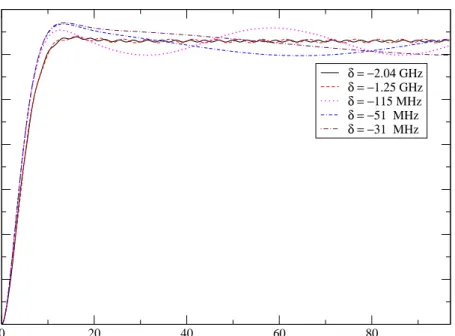
3.6 The coherent population oscillations for different detunings in the time domain for 1.47 nm diameter NCs with Es = 200 V /m, Ep = 20 V /m, and T2/T1 = 0.2. . . . 32
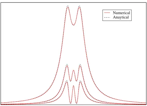
3.7 The comparison of numerical calculations with the analytical sults for arbitrary parameters. The absorption response with re-spect to detuning. . . 33 3.8 The comparison of numerical calculations with the analytical
sults for arbitrary parameters. The dispersive response with re-spect to detuning. . . 33 3.9 The absorptive response is given as a function of detuning and
for different T2
T1. For 1.47 nm diameter NCs, Es = 150 V /m and
Ep = 15 V /m. . . . 34 3.10 The imaginary part of susceptibility, χ is given as a function of
detuning and for different Es
Ep. For 1.47 nm diameter NCs, fixing
Ep = 15 V /m. . . . 35 3.11 The real part of susceptibility is given as a function of detuning and
for different Es
Ep. For 1.47 nm diameter NCs, fixing Ep = 15 V /m. 35
3.12 Slowdown factor versus the pump field intensity. For 1.47 nm diameter NCs, fixing Ep = 15 V /m. . . . 36 3.13 Slowdown factor versus the pump field intensity. For 2.01 nm
diameter NCs, fixing Es = 3000 V /m. . . . 37 3.14 Slowdown factor versus the phase difference between the pump and
probe fields. . . 38 4.1 Comparison of OBEs and SBEs when there is no Coulomb
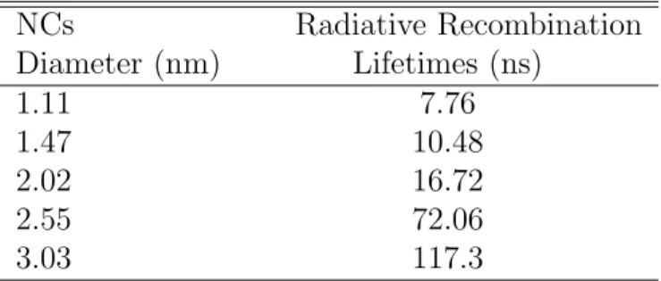
3.1 The radiative lifetimes for different NCs diameters. . . 31
Introduction
Nanocrystals (NCs) are nanometer-scale semiconductor crystals where the car-riers are spatially confined in all three dimensions. The quantum confinement effects breaks up the continuous density of states within the conduction and va-lence bands into discrete quantized states and leads to the discrete energy levels with sharp optical absorption spectra; similar to those of atoms and molecules. By these similarities, NCs are usually regarded as artificial solid-state atoms [1, 2, 3]. These similarities triggered numerous works to investigate the atomic-like properties in NCs. As expected atomic-like emission and absorption spectra of NCs observed in the early 1990s [4, 5, 6]. However, besides the atomic-like electronic and optical properties, NCs have several application advantages over the atomic systems. Since NCs are mesoscopic systems consisting of 103 to 106
individual atoms and molecules, there is a possibility of engineering the compo-sition, size and shape of NCs. As such, one can control the energy levels and optical properties of NCs. The robust structure of NCs at room temperature is also a significant advantage over the atomic systems which can be captured only for the short durations via complicated cooling and trapping techniques [1]. Moreover, crystalline effects such as carrier-carrier and carrier-phonon interac-tions bring new properties to NCs which are not available in atomic systems. These advantages can be employed for technological applications, provided that we understand the fundamental physics of the electronic and optical properties
associated with NCs.
In this thesis, we follow the trail of some fundamental atomic quantum co-herence effects on germanium (Ge) NCs. Besides their fundamental interest the quantum coherence phenomena are important for the applications such as the quantum computation [1] and slow light [7]. Our emphasis here is on the gener-ation of slow light in Ge NCs.
Ge NCs embedded in silica exhibit atomic-like states which are very conve-nient for the coherent control schemes. However, a more fundamental reason for our consideration of Ge NCs is due to their lowest unoccupied molecular or-bital (LUMO) level widely separated from the higher-lying states by more than 250 meV for NCs smaller than 2 nm; this property is unique and it is not the case for instance for silicon NCs [8]. Hence, this advantageous electronic structure of Ge NCs offers an ideal setting for exploring the quantum optical effects.
Figure 1.1: Energy spectra of germanium NCs of four different diameters em-bedded in a wide bandgap matrix computed with our atomistic pseudopotential approach; band edges of the bulk Ge is also marked as a reference [8].
In this computational expedition, aiming for a realistic account, the electronic structure and optical dipole matrix elements are computed using an atomistic pseudopotential approach; this is particularly challenging for a system containing
about several thousand atoms [9]. Figure 1.1 shows the evolution of the electronic states as the size of the Ge NCs varies; the widely-separated LUMO level for small diameters can be observed [8].
The velocity at which an optical pulse propagates through a material is given by the group velocity and expressed as,
νg =
c n + ωdn
dω
(1.1) where c is the group velocity of the light in vacuum, ω is the angular velocity of the pulse and n is the refractive index of the material [7]. As Eq. (1.1) indicates the group velocity depends not only on the refractive index, but also on the refractive index dispersion (i.e. dn
dω). Usually the dispersion is so small then the group velocity is equal to c
n. Nevertheless, the group velocity can be reduced to very small limits by exploiting the refractive index dispersion value.
Slow light is important both for fundamental understanding of quantum coher-ence effects and promising for new applications in quantum information and infor-mation processing such as all-optical networks, controllable optical data buffers, and optical data storage and memories. However, for such applications main aim is not just slowing the light but more essentially generating a tunable time delay by controlling the group velocity. The capacity of an optical buffer in an opto-electronic devise is directly proportional to the variability of the group velocity [10].
When an electromagnetic field is slowed down in a medium, its energy density increases. Since the nonlinear effects depend on the local energy density, the spatial compression of optical energy can be used to enhance the nonlinear optical effects. By this way, the nonlinear effects can be observed at much more lower applied powers than usually required [11].
The key to produce slow light is to give a mechanism which can lead to a transparency window in the absorption spectra. However, although, the medium is highly transparent, there is still a strong dispersion to produce slow light. Any mechanism that burns a hole in the absorption and gives rapid spectral variation of refractive index can produce slow light [12].
In 1992, Harris et al. [13] estimated that the electromagnetically induced transparency (EIT) can be used to generate slow light. EIT is a quantum in-terference effect fundamentally based on the coherent population trapping in a three level system. Experimental observation of this mechanism to slow the light was reported by Hau et al. [14]. They reported a group velocity of about 17 m/s in a Bose-Einstein condensate. Using EIT many groups observed slow light in different material systems [15, 16, 17].
For possible applications interest is eventually directed towards the room tem-perature solid materials. The problem with EIT in those systems is large dephas-ing rates compared with gases that broaden spectral features and preclude strong dispersion required for the production of slow light.
Bigelow et al. [18] suggested a new mechanism, the coherent population oscil-lation (CPO) to produce slow light in a solid state material at room temperature. Unlike EIT, this new mechanism relies on a two-level system for the propaga-tion material. They observed a group velocity of about 57 m/s in a ruby crystal at room temperature. Following their work, several other groups applied CPO mechanism to produce tunable slow light in semiconductor quantum wells and dots [19, 20, 32, 22].
CPO can be observed when a strong pump field and weak probe field with slightly different frequencies interact within a saturable absorber material. In this process the ground state population is induced to oscillate at the beat frequency between the pump and probe fields. When the beat frequency is smaller than or approximately equal to the inverse population relaxation time T−1
1 , the oscillation
can lead to a sharp decrease of the absorption of the probe field and so a rapid frequency variation of the refractive index experienced by the probe field. Since such a rapid variation means dn
dω > 0, by Eq. (1.1), gives rise to small group velocities for the probe field.
The advantage of CPO over EIT is the former required long population relax-ation times whereas the latter requires long dephasing times. In solid materials carrier-carrier and carrier-phonon scatterings give rise to very small dephasing times. Hence CPO is more adequate to implement slow light in the solid state
mediums. Actually we are going to see that short dephasing times are very crucial to generate the population oscillations.
In this Thesis, we use CPO to generate a transparency window within the absorption profile.
An analysis based on the atomic quantum theories does not give a complete description of semiconductor behavior, since the many-body interactions between the carriers are neglected. For a more realistic calculation the semiconductor effects should be included in a consistent manner. The inclusion of the many body effects into the atomic quantum coherence theory can be accomplished using the semiconductor Bloch equations [23]. The choice of nanocrystals becomes more meaningful in this sense since with their atomic-like properties NCs are best structures for the transition from atomic systems to semiconductors.
Due to the carrier-carrier scatterings, the redistribution of populations and the renormalization of energy levels are expected. Such contributions will modify the spectral shape and magnitude of quantum coherence effects [24]. When the many-body interactions are included to the calculations, the dephasing processes become significantly faster due to carrier-carrier and carrier-phonon collisions. Hence in order to maintain the coherence effects, higher coupling fields are re-quired.
The main result of Coulomb interaction is the carrier-carrier scattering. If the external driving fields do not vary much in the typical carrier-carrier scattering time of less then picoseconds, the scatterings just drives the electron and hole dis-tributions within each band to Fermi-Dirac disdis-tributions. Hence, carrier-carrier interactions can be included to the calculations by the effective rate approxima-tions which describe in which rate the population distribuapproxima-tions converge to the quasi-Fermi-Dirac distributions [25].
1.1
This Work
The organization of this Thesis is as follows:
In the following chapter we introduce the density matrix formalism of light-matter interaction and derive the optical Bloch equations for a multi-level system. The dephasing processes are included phenomenologically in terms of the relax-ation and dephasing times. Next, we discuss the two-level approximrelax-ation and present the analytical and numerical solution methods for the two-level OBEs.
In Chapter 3, we briefly describe our electronic structure calculations called linear combination of bulk bands (LCBB). Next, we illustrate that dephasing and relaxation times are very crucial inputs for the solutions of OBEs and thus we discuss the range of these values for Ge NCs. While solving OBEs for Ge NCs, we explain the hole burning phenomena and represent our results for slow light production in Ge NCs. We give the size-scaling of slow-down factor with respect to NC diameter and Stark effect.
In Chapter 4, we develop an analysis which explains the semiconductor quan-tum coherence phenomena in Ge nanocrystals. Due to the strong many-body ef-fects, some deviations from the results of atomic coherence theory are inevitable. In that part, we treat the light-matter interaction in terms of second quantized electron-hole formulation. The semiconductor Bloch equations are introduced to investigate quantum coherence phenomena in semiconductors. The carrier-carrier and carrier-phonon interactions are included in the context of Hartree-Fock ap-proximation. The collision effects beyond that approximation are added in terms of effective relaxation rates.
Chapter 5 contains the conclusion which gives aa brief discussion of all the preceding chapters and results of SBEs are expected as a future work.
Optical Bloch Equations
In the present chapter we derive the density matrix formulation of the light-matter interaction. We consider the interaction for a multi-level system. After deriving the general formalism, we are going to concentrate on the physics of two-level scheme. A two-level approximation is useful when the two-levels of the interest to the medium are in resonance nearly with the applied fields whereas all the other levels are significantly detuned.
2.1
General Formalism
Quantum mechanically, one can specify the dynamic state of a single particle in terms of its state function. Similarly the dynamics of a quantum mechanical system can be specified in terms of a pure state function. On the other hand, in order to describe the state of a macroscopic medium containing many particles we need the complete knowledge of states of all the particles in the medium. In such a case we can apply the statistical mechanics in order to calculate the averaged expectation values of observable medium quantities. That is, we consider the probability distribution function Pi over all the possible states |ψii of the system. Then the expectation value of some physical quantity represented by the operator
ˆ
O is averaged over the all possible states and given by h ˆOi =X
i
Pihψi| ˆO|ψii , (2.1)
where |ψii is a state of the complete set of orthonormal quantum states of many-particle system. The right hand side of Eq. (2.1) can be written in the matrix representation using an arbitrary complete basis set |ni,
h ˆOi =X n,m X i Pihψi|nihn| ˆO|mihm|ψii . (2.2) Rearranging terms h ˆOi = X n,m " X i Pihm|ψiihψi|ni # hn| ˆO|mi , (2.3)
which can be written as
h ˆOi = X
n,m
hm|ˆρ|nihn| ˆO|mi , (2.4)
where we defined the element of a matrix, called the density matrix
ρmn = hm|ˆρ|ni =
X
i
Pihm|ψiihψi|ni , (2.5) and the corresponding density operator is
ˆ
ρ ≡X
i
Pi|ψiihψi| . (2.6)
Then Eq.(2.4) will be
h ˆOi =X
m
hm|ˆρ ˆO|mi = tr(ˆρ ˆO) , (2.7) where we used tr, trace that is the sum of the diagonal elements and invariant to any unitary transformation of the representation. Hence the expectation value is independent of any specific representation. Let us here make a remark that as long as our equations are linear, we can effectively replace the operators in equations by their expectation values, i.e., ˆρnm → hˆρnmi ≡ ρnm. This can be performed by taking the expectation values of both sides of equations. Hence we drop the hats of operators, since their meanings can be understood from the content.
The elements of density matrix have significant physical interpretations. Con-sider for example, our multi-level system of light-matter interaction. The diagonal
matrix elements are real by Eq. (2.5), ρnn =
X
i
Pi|hn|ψii|2, (2.8)
where the probability, that a particle in the state |ψii will be found in the level
|ni is averaged over all the states occupied by the particles of the medium. Hence
this value corresponds to the population distribution on the level |ni.
On the other hand, the off-diagonal elements ρnm are the averages of the product of the expansion coefficients hn|ψii and hm|ψii, and they have a complex conjugate property ρnm = X i Pihn|ψiihψi|mi = X i Pi∗hm|ψii∗hψi|ni∗ = ρ∗mn. (2.9) Since the expansion coefficients are complex in general, we can write them as amplitudes and phases
ρnm =
X
i
Pi
h
|hn|ψii||hψi|mi|ei(φn−φm)
i
. (2.10)
If neither of the expansion coefficients is equal to zero, then whether the off-diagonal elements vanish or not will depend on whether the relative phase factor (φn − φm) averages to zero or not. If the wave functions are incoherent with randomly distributed relative phases, then the off-diagonal elements average to zero. So the off-diagonal element ρnm is a measure of the coherence between the levels n and m, in the sense that it will be nonzero if the system is in a coherent superposition of energy eigenstates |ni and |mi.
We can understand the significance of coherence considering the macroscopic electric polarization of a medium via induced dipole moment. The macroscopic polarization is given as
~
P = Nh~µi , (2.11)
in terms of the expectation value of dipole moment µ where N is the dipole number density of the medium. The dipole matrix elements are
where −e is the electron charge and ˆr is the position operator for the electron.
By the assumption that the wave functions corresponding to states |ni and |mi have definite parity, the diagonal elements hn|ˆr|ni vanish as a consequence of
symmetry considerations. It also means that the medium has no permanent dipole. Consider for the sake of clarity the expectation value of dipole moment for a two-level system, h~µi = tr(ρ~µ) where ρ~µ is represented as
h~µi = tr(ρ~µ) = tr ρ11 ρ12 ρ21 ρ22 0 ~µ12 ~µ21 0 = tr ρ12~µ21 ρ11~µ12 ρ22~µ21 ρ21~µ12 , (2.13) thus the expectation value of dipole moment is
h~µi = tr(ρ~µ) = ρ12~µ21+ ρ21~µ12. (2.14)
Hence, we observe that the expectation value of the dipole moment depends on the off-diagonal elements of the density matrix. That is, the off-diagonal elements are a measure of the macroscopic polarization of the medium. This illustrates the importance of off-diagonal elements since from the polarization we can switch to other macroscopic properties of the medium [24].
For future reference, combining Eqs. (2.11) and (2.14), we obtain the macro-scopic polarization in terms of dipole moments and density matrices,
~
P (t) = N [ρ12(t)~µ21+ ρ21(t)~µ12] , (2.15)
where N is again the density of dipole moments. On the other hand, the linear polarization in the frequency domain is related to the complex susceptibility of the medium by
~
Pi(ω) = ²bχij(ω)~Ej(ω) (2.16) where the subscripts i and j indicate the Cartesian components and ²b is the host material dielectric constant [39]. In an anisotropic medium, χ is a tensor. However, in the homogeneously spherical NCs it turns out just a scalar quantity. After a Fourier transformation, the macroscopic polarization given in Eq. (2.15) can also be written in the frequency domain. This gives rise to the relation [39],
~
from which we can extract the susceptibility, ˜
χ(ω) = N [ρ12(ω)~µ21+ ρ21(ω)~µ12] ²bE(ω)~
. (2.18)
The propagation of an electromagnetic field in a dispersive medium can be characterized by the frequency dependent complex susceptibility, χ = χ0+iχ00. We assume small field amplitudes so that the medium displays only linear response. The imaginary part of the susceptibility, χ00 gives the absorption of the medium whereas the real part, χ0 corresponds to the dispersion of the medium [27]. We will return to these discussions when we are ready to solve density matrices in the frequency domain.
Hence in summary, the diagonal elements of density matrix give the relative populations of energy levels and the off-diagonal elements, in our case, takes part in the calculation of polarization. The dynamics of the multi-level system, thus the evolution of populations and polarization over time can be described by the time dependence of the density matrix.
From the definition of ρ, we can observe that it can evolve in time by two reasons. One is the time dependence of the probability function Pi(t) of the state
|ψii. Other is the time-dependence of the state function |ψii, itself. Thus we can write the time evolution of ρ by using its definition given by Eq. (2.6),
d dtρ = X i "à ∂ ∂t|ψi(t)i ! Pihψi| + |ψii à ∂ ∂tPi(t) ! hψi| + |ψiiPi à ∂ ∂thψi(t)| !# . (2.19) Assume that our system has no relaxation process or no random forces, i.e., all the particles experience the the same forces. So all the particles in the medium can be described by the same Hamiltonian. That is in the absence of relaxation processes, the probability of each state conserved and the probability distribution function Pi does not change explicitly with time,
∂
∂tPi = 0 . (2.20)
Since we stated that all the particles have the same Hamiltonian, then by the Schr¨odinger Equation ∂ ∂t|ψi(t)i = − i ¯hH|ψi(t)i and ∂ ∂thψi(t)| = i ¯hhψi(t)|H . (2.21)
Inserting Eqs. (2.20) and (2.21) into (2.19) we obtain the equation of motion for ˆ
ρ in the absence of relaxation processes,
˙ρ = −i
¯h[H, ρ] . (2.22)
This equation is known as the Liouville equation which describes the time evolu-tion of density operator.
So far we excluded the relaxation processes which are always present in real media. The randomizing forces corresponding to the relaxation processes (such as collisions between particles) act differently on each particle. Since there is no way of calculating exactly these random forces, they may be approximated phenomenologically. We expect a general form of
˙ρ = −i ¯h[H, ρ] + Ã ∂ρ ∂t ! rel , (2.23)
where the term (∂ρ/∂t)relreflects the relaxation effects since our condition of Eq. (2.20) is not valid any more. The relaxation can be included to the formalism in several ways. Rigorously one can introduce the master equation which contains system-reservoir interactions, then solve the corresponding equations of motions [37, 38]. Nevertheless, the reasoning of that method indicates that the relaxation processes can be described quite well by adding phenomenological damping terms to the density matrix equation,
˙ρnm= − i ¯h[H, ρ]nm− γnm ³ ρnm− ρ(eq)nm ´ , (2.24)
which means if the medium is not too far from thermal equilibrium, ρnmrelaxes to its equilibrium value ρnm at rate γnm. When the system is in thermal equilibrium the excited states may contain population, i.e., ρ(eq)
nm can be nonzero. However, the thermal excitation is expected to be an incoherent process so that cannot produce any coherent superposition of states. Thus the off-diagonal elements average to zero, ρ(eq)
nm = 0 for n 6= m. Since γnm is a decay rate, we can also write
γnm = γmn.
Alternatively, in a different approach, for the diagonal elements we may allow population decays from higher levels to lower levels. Assuming above discussion
still describes the off-diagonal elements, we write the density matrix equations, ˙ρnm = − i ¯h[H, ρ]nm+ X Em>En Γnmρmm− X En>Em Γmnρnn, (2.25) where Γnm is the rate of population decay from level |mi to level |ni, and Γnm is the damping rate of γnm coherence. The diagonal and off-diagonal damping rates are related in a way
γnm = 1
2(Γn+ Γm) + γ
(pro)
nm , (2.26)
where Γn and Γm are the total decay rates of population out of levels |ni and
|mi, respectively, i.e.,
Γn=
X
En>En0
Γn0n, (2.27)
and γ(pro)
nm is the proper dephasing rate which collects the dephasing processes that are not related with the population transfer such as collisions.
We can relate above relaxation rates with relaxation times which are more explicit for us. Following the first approach to the relaxation processes, in the language of quantum optics, the diagonal relaxation rates corresponds to popu-lation relaxation time of level |ni, γ−1
nn = Tnn. The off-diagonal relaxation rates correspond to polarization dephasing time, γ−1
nm= Tnm. Its name originates from Eqs. (2.11-2.14) since dipole moment dephases in this characteristic time. In a two-level system Tnn and Tnmare usually denoted as T1 and T2 or for a multi-level
system (T1)nn and (T2)nm, respectively. T1 and T2 terminology originates from
the magnetic resonance phenomena in which literature T1-time is referred to as
longitudinal relaxation time and T2-time is referred to as transverse relaxation
time [40].
Due to energetic considerations, it is always easier to change the phase rather than altering the populations in a relaxation process so that T2 is always shorter
than corresponding T1. The difference in relaxation times, their values and their
comparison with other system parameters give rise to important physical conse-quences as we are going to see in the following sections.
2.2
Multi-Level System
So far we introduced the general idea of density matrix equation. Now we can specify this equation for the light-matter interaction problems. Let us rewrite the density matrix equation of motion that we are supposed to solve,
˙ρnm = − i ¯h[H, ρ]nm− ρnm− ρ(eq)nm Tnm . (2.28)
First, consider the absence of external perturbation and relaxation processes. In such a case the density matrix equation gets the form
˙ρnm = −
i
¯h[Ho, ρ]nm . (2.29)
Since there is no perturbation, we can assume that the time-independent Schrodinger equation
Ho|ni = En|ni , (2.30)
can be solved. For our multi-level system this will give the interaction-free ener-gies of levels, i.e., En= ¯hωn. Thus we can write
˙ρnm = − i ¯h[Ho, ρ]nm= − i ¯h(Hoρ − ρHo)nm = − i ¯h X j (Ho,njρjm− ρnjHo,jm) = −i ¯h X j (Enδnjρjm− ρnjδjmEm) = −i ¯h(Enρnm− Emρnm) = −iωnmρnm, where we defined the transition frequency ωnm≡ (En− Em)/¯h.
Next, if we subject the medium to a time-dependent external perturbation, the total Hamiltonian will be
H = Ho+ V(t) , (2.31)
where the operator V(t) represents the perturbation and Ho is the unperturbed Hamiltonian. Then the density matrix equation is
˙ρnm= − i ¯h[H, ρ]nm = − i ¯h[Ho, ρ]nm− i ¯h[V, ρ]nm , (2.32) where we can write
[V, ρ]nm = (Vρ − ρV)nm =
X
j
For the interaction of electromagnetic radiation with an optical medium, we can specify the perturbation using the electric dipole approximation,
V(t) = −~µ · ~E(t) , (2.34)
where ~µ is the electric dipole moment. In this approximation it is assumed that the wavelength of the electromagnetic field is much larger than the size of medium. So the amplitude of the field does not vary across the medium. This allows us to write ~E(z, t) → ~E(t). We also ignore the effects of magnetic field [41]. Following
Eq. (2.12), the matrix representation of interaction potential is given as
Vnm= Vmn∗ = −~µnm· ~E(t) . (2.35)
For the electromagnetic field, we are going to use a pump-probe scheme. In pump-probe experiments, a strong pump field and a weak probe field excites the medium simultaneously [42]. The frequency of the probe field is going to be scanned around the frequency of the pump field. Working within the framework of semiclassical laser theory, we treat the applied fields classically and the medium quantum mechanically. So we write the total bichromatic field as
~
E(t) = ~Ese−iωst+ ~Epe−iωpt+ ~Es∗eiωst+ ~Ep∗eiωpt, (2.36) where Ei are complex amplitudes, ωi is the frequency and the subscripts s and p identify the strong pump and weak probe fields.
Finally including the relaxation times we can write the general form of density matrix equation of motion for the optical medium coupling to electromagnetic fields, ˙ρnm= −iωnmρnm− ρnm− ρ(eq)nm Tnm + i ¯h X j ³ ~µnj· ~E(t)ρjm− ρnj~µjm· ~E(t) ´ . (2.37)
We can further specify n and m values, and solve the resulting density matrix equations. Let us consider the two-level model.
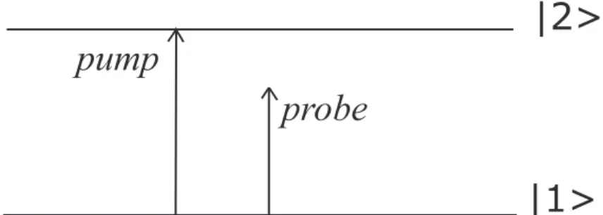
|2>
|1>
probe
pump
Figure 2.1: Two-level model
2.3
Two-Level System
We consider a two-level system. The lower level is denoted |1i and the upper level |2i as illustrated in Fig. 2.1. In Eq. (2.37) we run n and m values over 1 and 2 to obtain the density matrix equations of the system,
˙ρ21 = −iω21ρ21− ρ21 (T2)21 + i ¯h ³ ~µ21· ~E(t)ρ11− ρ22~µ21· ~E(t) ´ , (2.38) ˙ρ11 = − ρ11− ρ(eq)11 (T1)11 + i ¯h ³ ~µ12· ~E(t)ρ21− ρ12~µ21· ~E(t) ´ , (2.39) ˙ρ22 = −ρ22− ρ (eq) 22 (T1)22 + i ¯h ³ ~µ21· ~E(t)ρ12− ρ21~µ12· ~E(t) ´ , (2.40)
where we used the results of previous part such that ρ(eq)
nm = 0 for n 6= m and
µnn = 0 by the parity of wave functions. Due to the relation ρ12 = ρ∗21 that we
showed in Eq. (2.9), no separate equation is required for ρ12.
In a closed two-level system, the total population ρ22+ ρ11 is conserved. This
means that a decrease in one population should cause an increase in the other population, or vice versa. This gives rise to ˙ρ22+ ˙ρ11= 0 and since Tnm = Tmn we can write (T1)22 = (T1)11≡ T1. By the same reason, for the coherence dephasing
times we have (T2)21= (T2)12 ≡ T2.
Since Eq. (2.38) depends on the populations ρ22 and ρ11 by their difference
difference ρ22− ρ11. Subtracting Eq. (2.39) from Eq. (2.40) we obtain ˙ρ22− ˙ρ11 = − (ρ22− ρ11) − (ρ22− ρ11)(eq) T1 +2i ¯h ³ ~µ21· ~E(t)ρ12− ρ21~µ12· ~E(t) ´ . (2.41) For the electric field we use Eq. (2.36), thus we obtain the optical Bloch equations (OBEs) for a two-level system,
˙ρ21= − µ iω21+ 1 T2 ¶ ρ21− i ¯h−→µ21· h ~
Ese−iωst+ ~Epe−iωpt+ ~Es∗eiωst+ ~Ep∗eiωpt
i (ρ22− ρ11) , (2.42) ( ˙ρ22− ˙ρ11) = − (ρ22− ρ11) − (ρ22− ρ11)(eq) T1 + 2i ¯h~µ21· h ~
Ese−iωst+ ~Epe−iωpt+ ~Es∗eiωst+ ~Ep∗eiωpt
i ρ12 − 2i ¯h~µ12· h ~
Ese−iωst+ ~Epe−iωpt+ ~Es∗eiωst+ ~Ep∗eiωpt
i
ρ21. (2.43)
Now we are supposed to solve these coupled equation in order to understand the response of the two-level system to the pump-probe fields. The usual way of solution is applying an analytic method which was extensively discussed in the classical paper [27] and also can be found in [26],[11] and [7]. We solved the density matrix equations numerically without their approximations. Their solutions are valid for the steady state with the approximation of treating the strong field Es correctly to all orders while treating the weak field Ep to only first order. Under this assumption they observe by inspection that the solution of Eqs. (2.42-2.43) for ρ22(t) − ρ11(t) will have the form,
ρ22(t) − ρ11(t) = (ρ22− ρ11)(0)+ (ρ22− ρ11)(δ)e−iδt+ (ρ22− ρ11)(−δ)eiδt, (2.44)
where δ ≡ ωs− ωp is the beat frequency. This equation illustrates that the popu-lation difference of two levels has components oscillating with the beat frequency. This oscillatory behavior of populations is called the coherent population oscilla-tions (CPO). To observe the oscillaoscilla-tions the population relaxation rate γ1 = 1/T1
should be larger compared with the beat frequency, δ.
In steady state solution [7, 11, 27] the transition element of density matrix ρ21
and m are integers. With the above approximation that the probe field Ep is weak and treated only to first order whereas the pump field Es is strong and treated to all orders, it is also observed by inspection of Eqs. (2.42-2.43) that the solution for ρ21(t) oscillates dominantly at three frequencies: ωs, ωp, and 2ωs− ωp. Thus the steady state solution for ρ21(t) can be expressed as following Ref. [27],
ρ21(t) = ρ21(ωs)e−iωst+ ρ21(ωp)e−iωpt+ ρ21(2ωs− ωp)e−i(2ωs−ωp)t, (2.45) where ρ21(ωi) are called Fourier amplitudes and defined as
ρ21(ωs) = Ωs(ρ22− ρ11)dc 2(ωs− ω21+ i/T2) , (2.46) ρ21(ωp) = Ωp(ρ22− ρ11)dc 2D(ωp) · µ ωp− ωs+ i T1 ¶ µ ωp − 2ωs+ ω21+ i T2 ¶ − Ω 2 s(ωp− ωs) 2(ωs− ω21− i/T2) ¸ , ρ21(2ωs− ωp) = Ω2 sΩp(ρ22− ρ11)dc(ωp− ωs+ 2i/T2) 4D(ωp)(ωs− ω21− i/T2) , (2.47)
where Ωi = 2|Ei||µ21|/¯h is the on-resonance Rabi frequency for the electric field
of amplitude 2Ei and (ρ22− ρ11)dc the steady-state saturated population inversion
induced by the pump field Es is defined as (ρ22− ρ11)dc = [1 + (ωs− ω21)
2T2
2] (ρ22− ρ11)0
1 + (ωs− ω21)2T22+ Ω2sT1T2
, (2.48)
and the so called cubic function, D(ωp) is
D(ωp) = (ωp−ωs+i/T1)(ωp−ω21+i/T2)(ωp−2ωs+ω21+i/T2)−Ω2s(ωp−ωs+i/T2) .
(2.49) The physical meanings of Fourier amplitudes are important. The final one
ρ21(2ωs − ωp) gives rise to generation of a field with frequency ω = 2ωs− ωp. If a wave with this frequency already exist in the medium than it may be ampli-fied. Similarly ρ21(ωs) and ρ21(ωp) give rise to absorption or amplification of the pump and probe fields, respectively. For our purposes the amplitude ρ21(ωp) is the crucial term.
In the mathematical language, the density matrix Eqs. (2.42-2.43) are coupled first-order differential equations which can be solved numerically with several
different methods to obtain ρ21(t) and ρ22(t) − ρ11(t) [28]. We preferred the
fourth order Runge-Kutta method [28]. The relaxation times are on the orders of nanoseconds for Ge NCs. For such relaxation times, time steps on the order of 10 ps produce proper results. In order to obtain smooth absorption curves, we observe the system up to 50 µs time range.
Since we are mainly interested with ρ21(ωp), we should switch from ρ21(t) to
ρ21(ω). This can be done by Fourier transformation of ρ21 from time space to
frequency space. We get the Fourier transform as
ρ21(ω) = 1 2π Z ∞ −∞ρ21(t)e iωtdt . (2.50)
Nonetheless, for our purposes we do not need the whole spectrum of ω for ρ21
since we are interested just in ρ21(ωp). Thus we can set ω = ωp in Eq. (2.50) to get ρ21(ωp) = 1 2π Z ∞ −∞ρ21(t)e iωptdt . (2.51)
This was the theoretical discussion of Fourier transformation, but computation-ally of course we can not run (−∞, +∞) interval. Since the response starts at
t = 0, we have ρ21(t < 0) = 0. That brings the lower limit of integration from
−∞ to zero. For the upper limit, we should cut the integration at a sufficiently
long time t = T . This is physically meaningful because our system of light-matter interaction converges to a steady state rapidly. Following the theory of Fourier transformation since our limits of integration changed from (−∞, +∞) to (0, T ), we should also change the 1/2π coefficient of integration by 1/T , thus finally we get ρ21(ωp) = 1 T Z T 0 ρ21(t)e iωptdt . (2.52)
Although, the OBEs given in Eqs. (2.42) and (2.43) can be solved while in those forms, the rapid oscillatory behavior of exponential parts increases the calculation time. In order to simplify the calculations, we see from Eq. (2.42) that the nondriven (i.e., E(t)) behavior of ρ21 is ρ21(t) = ρ21(0)e−(iω21+1/T2)t so
that, for ωp ≈ ω21, it is useful to introduce some slowly varying variables σ21 and
σ12 as
ρ12(t) = ρ∗21(t) = σ12(t)eiωpt, (2.53)
inserting these new variables into OBEs, we get: ˙σ21= − · i(ω21− ωp) + 1 T2 ¸ σ21− i ¯h~µ21· h ~ Ese−i(ωs−ωp)t+ ~Ep i (ρ22− ρ11) , (2.54) ( ˙ρ22− ˙ρ11) = − (ρ22− ρ11) − (ρ22− ρ11)(eq) T1 + 2i ¯h~µ21· h ~ Ese−i(ωs−ωp)t+ ~Ep i σ12 − 2i ¯h~µ12· h ~ E∗ sei(ωs−ωp)t+ ~Ep∗ i σ21, (2.55)
where we eliminated terms with time dependence e±i(ωs+ωp)t and e±i2ωpt, since
they oscillate rapidly and their contribution averages to zero in a short time compared to that of observation. This approximation is called the rotating wave approximation (RWA). Although, such an implementation lengthen the analytical derivations, it reduces the computation times on the order of more than 105.
Notice that by the definition of new operator σ, the transform given in Eq. (2.52) gets a simpler form,
ρ21(ωp) = 1
T
Z T
0 σ21(t)dt . (2.56)
Above Eqs. (2.54) and (2.55) explicitly manifest that the dynamics of a opti-cally excited system is determined by population relaxation time T1and dephasing
time T2. Since the population relaxation also implies the phase relaxation of the
optically excited dipoles, T1 should be related to T2, the decay of interband
po-larization. In the absence of collisional decays, the population lifetime of excited state, T1 is twice the coherence dephasing time, T2, i.e.,
1
T2
= 1
2T1
, (2.57)
for a two-level system [2, 3]. So this relation holds in the case of pure dephasing due to the finite lifetime of excited state. In general, different phase destroying processes are involved in dephasing dynamics giving a sum over different times
Ti, 1 T2 = 1 2T1 +X i 1 Ti . (2.58)
These phase destroying processes are the coupling to different types of phonons, phase destroying scattering between carriers in a interacting many-body system and scattering at defects or interfaces [2]. It is difficult to determine different process times but in any case Eq. (2.58) comprises the relation
T2
T1
≤ 2 , (2.59)
which actually sets an upper limit for T2 since population relaxation always leads
to dephasing of coherence.
So far we obtained the optical Bloch equations for a two-level system. In the next chapter we implement our derivations to the Ge NCs.
Slow Light in the Optical Bloch
Equations Level
When we consider the OBEs, Eqs. (2.54) and (2.55) derived in the preceding chapter, we notice that the medium material is described in the equations via the energy levels, electric dipole moments, and relaxation and dephasing times. In this chapter, first of all we briefly introduce our electronic structure calculations. Then we discuss the relaxation and dephasing times for Ge NCs. Finally, we solve the OBEs for Ge NCs and interpret the results within the context of slow light.
3.1
Electronic Structure Calculations
For the electronic structure calculations of large-scale nanostructure systems Wang and Zunger developed the linear combinations of bulk bands (LCBB) method [44]. The method introduces an effective calculation for the single-particle electronic states of million-atom nanostructure systems. The approach is funda-mentally based on an empirical pseudopotential Hamiltonian. After calculating the electronic structure for bulk constituent materials, the wave functions of the nanostructure is expanded in terms of bulk Bloch states of the constituent mate-rials. The expansion is performed over the bulk band indices, n and wave vectors,
k defined within the first Brilloin zone of a computational supercell which is pe-riodic in all three dimensions. This choise economizes the basis size compared to plane wave type of approaches.
The main advantage of LCBB is very small calculation time of electronic structure even for million-atom nanostructures. Note that ab initio calculations are still science fiction for atomic systems containing more than 1000 atoms.
The main ingredients of LCBB are the atomic positions and the atomic pseu-dopotentials. The method gives the atomistic level wave functions which let us calculate the Coulomb interaction explicitly. Our bulk electronic structure cal-culations are based on the empirical pseudopotential method (EPM) which is also very fast, accurate and easy to implement [45, 46]. Moreover, particularly unlike ab initio calculations, EPM agrees with the experimental bandgap very accurately by its construction.
While implementing the LCBB method, we expand the jth state NC wave function in terms of the linear combinations of bulk Bloch bands of the constituent core and embedding medium materials,
ψj(~r) = 1 √ N X n,~k,σ Cσ n,~k,je i~k·~ruσ n,~k(~r) , (3.1)
where N is the number of primitive cells in the supercell and the superscript σ indicates the core or embedding medium materials. uσ
n,~k(~r) is the cell-periodic part of the Bloch states and can be expanded by the plane wave functions of reciprocal-lattice vectors { ~G} as uσ n,~k(~r) = 1 √ V0 X ~ G Bσ n~k ³ ~ G´ei ~G·~r, (3.2)
where V0 is the volume of the primitive cell.
Our demand is to determine the expansion coefficients Cσ
n,~k,j defined in Eq. (3.1). For that we start by writing the single-particle atomistic pseudopotential Hamiltonian of the system,
ˆ H = −¯h 2∇2 2m + X σ, ~Rj,α Wσ α( ~Rj) υσα ³ ~r − ~Rj − ~dσα ´ , (3.3)
where m is the free electron mass, ~Rj is the position of the primitive cell and
~ dσ
α gives the relative coordinate of atom of type (σ, α) within the primitive cell. The weight function Wσ
α( ~Rj) takes values 0 or 1 depending on whether an atom of type α is located at the position ~Rj + ~dσα. The screened spherical atomic pseudopotential υσ
α is determined by reproducing a large variety of empirical results such as bulk band structures, effective masses, and deformation potentials.
Then the coefficients Cσ
n,~k,j can be obtained by solving the following eigenvalue equation [44, 47]: X n,~k,σ Hn0~k0σ0,n~kσCn,~kσ = E X n,~k,σ Sn0~k0σ0,n~kσCn,~kσ , (3.4) where Hn0~k0σ0,n~kσ ≡ D n0~k0σ0| ˆT + ˆV xtal|n~kσ E , D n0~k0σ0| ˆT |n~kσE= δ ~k0,~k X ~ G ¯h2 2m ¯ ¯ ¯G + ~k~ ¯¯¯2Bσ0 n0~k0 ³ ~ G´∗Bσ n~k ³ ~ G´ , D n0~k0σ0| ˆV xtal|n~kσ E = X ~ G, ~G0 Bσ0 n0~k0 ³ ~ G´∗Bσ n~k ³ ~ G´ ×X σ00,α Vασ00µ¯¯¯G + ~k − ~~ G0− ~k0¯¯¯2 ¶ ×Wασ00³~k − ~k0´ei(G+~k− ~~ G0−~k0)· ~dσ00α , Sn0~k0σ0,n~kσ ≡ D n0~k0σ0|n~kσE .
while implementing this eigenvalue equation we assumed both the constituent core and embedding medium to have the same lattice constant. They are placed within a computational supercell which satisfies the periodicity condition W ( ~Rn1,n2,n3 +
Ni~ai) = W ( ~Rn1,n2,n3).
In this work, the constituent core material is Ge whereas for the embedding medium instead of a free-standing NC, we used an artificial wide band-gap mate-rial which satisfies the Ge/SiO2 band alignment. We set the lattice constant and
crystal structure of the embedding material equal to the diamond Ge to overcome the actual strain effects.
Within this method, we obtained the electronic structure and wave functions for different size Ge NCs (recall Fig. 1.1). Using the wave functions and Eq. (2.12), we calculated the electric dipole matrix elements. These quantities are required in order to solve OBEs for Ge NCs. Besides the electronic structure (i.e., energy levels of states) and electric dipole matrix elements, dephasing and relaxation times specifies the OBEs for a specific material.
Before presenting our results, we should give further technical preliminaries. As we are going to see in the Results part, in some cases when the probe field gets close to pump field its absorption decreases. This sharp dip in the absorption curve is called as hole burning.
3.2
Hole Burning
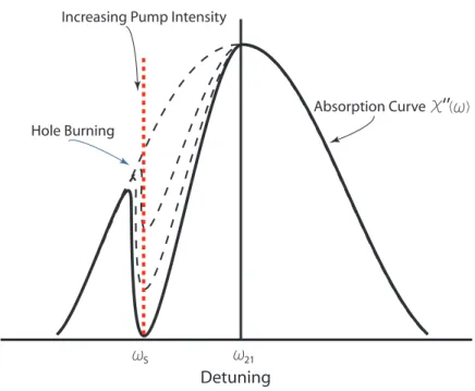
Hole burning in homogeneously saturable absorbers is an interesting property. Indeed at the early times of hole burning, it was commonly believed that the hole burning was a property of just inhomogeneous broadening [29, 30]. Consider an inhomogeneous medium with different excitation energies. When a probe field is applied to this medium with varying frequency, the absorption of the field will be a classical Lorentzian lineshape which means that the field experiences higher absorption in the vicinity of resonant transitions. However, if a strong pump field is applied to this medium in addition to weak probe field, the pump field will saturate the population differences whose transition frequencies are nearly in resonance with the pump field (see Fig. 3.1). The transitions at highly detuned frequencies will be untouched. Now with increasing power of this pump field, a sharp hole appears in the absorption line of the probe field. This hole is burned by the pump field in the vicinity of its frequency. The absorption of the probe field sharply decreases at the frequencies close to that of the pump field since those transitions are already saturated due to Pauli blocking by the strong pump field [30, 31, 32].
Increasing Pump Intensity Absorption Curve Hole Burning ω21 ωS χ‘’( ω) Detuning
Figure 3.1: Saturation of absorption in an inhomogeneous transition.
On the other hand, it is commonly believed that for the homogeneous broad-ened transition, the increasing strength of pump field will further saturate the probe field absorption uniformly without changing its shape or linewidth and cannot have such a hole, see Fig. 3.2. However, the hole burning effect in a pump-probe experiment for a homogeneously broadened medium was first ob-served by Soffer and McFarland [33] in 1966 and explained by Schwarz and Tan [26] in 1967. They and many other authors [34, 35] attributed the origin of such a hole to the periodic modulation of the ground state population at the beat frequency δ = ωs− ωp between the pump and probe fields. As we mentioned in
the previous section this phenomenon is called as coherent population oscillation (CPO). If the beat frequency between the fields is less than or approximately equal to the inverse of the population relaxation time T−1
1 then the population
can follow the oscillations of optical intensity and the absorption of the probe field will decrease (see Fig. 3.3). We have T1 here since it is the timescale within
which the population oscillation can follow the beating induced by the fields. Boyd and Mukamel [34] studied the theory of pump-probe experiment via
Detuning (ωs-ωp)
Absorption
Increasing pump intensity
Figure 3.2: Saturation of absorption in a homogeneous transition.
the nonlinear susceptibility χ(3). They showed that the general assumption of
pump-probe experiments that the pump field prepares the system and then a nonsaturating weak probe field monitors the system is not accurate enough to calculate the probe field absorption. In the sequential treatment of the fields, one first calculates the steady state just under the effect of pump field and then calculates the response of perturbed system to the probe field [36]. However, they showed that the sequential treatment omits the interference terms between the two fields which give rise to the hole burning in the probe absorption profile. They calculated a contribution term to the usual absorption which results in a dip in the lineshape. Keeping this remark in mind, we solve the density matrix equations applying both fields simultaneously.
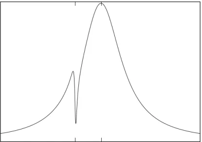
Although one can burn a hole on any region of the absorption spectrum (see Fig. 3.4), the deepest hole can be burned at the maximum of absorption spectrum. This means that the location of the spectral hole follows the frequency of pump field. Hence, the pump field does not need to be frequency locked to any specific transition. In order to get the maximum efficiency, we set the frequency of pump field in resonance with the difference between the HOMO-LUMO levels.
ωs Detuning (ωs -ωp)
Absorption
Without pump
With pump
Figure 3.3: This population oscillation becomes significant when the detuning is smaller than the inverse of population lifetime and gives rise to an absorption dip on the absorption profile.
ωs ω21 Detuning (ωp -ωs )
Absorption
ωs Detuning (ωs-ωp)
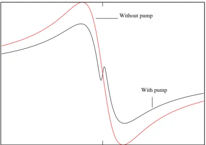
Real part of refractive index
With pump Without pump
Figure 3.5: Variation of the refractive index by pump application.
A dip in the absorption spectrum has significant consequences such as satura-tion spectroscopy [30] and manipulasatura-tion of the speed of light. Since the absorpsatura-tion hole has a width of 2T1−1, this effect has been employed to measure the population
lifetime in the saturation spectroscopy. The slow light is our next discussion.
3.3
Slow Light
The Kramer-Kronig relations, a consequence of causality condition, relate the absorption to the real part of the refractive index [7]. By this relation a narrow dip in the absorption spectrum will lead to a variation of the refractive index spectrum with a positive slope in the same frequency range, i.e., ∂n
∂ω > 0 (see Fig. 3.5). The induced population oscillation gives rise to a new polarization component thus alters the susceptibility and the refractive index experienced by the probe field.
of group velocity also given in the Chapter 1, vg = dω dk = c n + ω∂n ∂ω (3.5) where c is the speed of light in vacuum and n is the refractive index [7]. As we mentioned earlier, the large values of the refractive index dispersion can give rise to very small group velocities.
On the other hand, if we consider the opposite case, a narrow peak in the absorption spectrum corresponds to a large negative slope and produce superlu-minal (vg > c) light propagation [7]. Despite the name superluminal, there is no contradiction with the second postulate of special relativity since no information can be sent faster than c, the speed of light in vacuum [48].
Following the definition of group velocity, we can also introduce the slowdown factor defined as
S = c vg
= n + ω∂n
∂ω , (3.6)
which is indeed equal to the group index.
The refractive index is defined in terms of the dielectric function ² as,
n = v u u t q
Re{²}2+ Im{²}2+ Re{²}
2 , (3.7)
where the dielectric function is given by
² = ²b+ LLF Eχ. (3.8)
where ²b is the inert background dielectric constant which is taken in this work as ²b = 16 of Ge [8]. By LLF E, we include the surface polarization effects, also called local field effects (LFEs) to our calculations using a simple semiclassical model [9]. The effect is a result of the dielectric mismatch between the constituent NC and host matrix which lead to remarkably different optical properties. The correction factor LLF E for a linear response is given by,
LLF E =
3²h
²N C + 2²h
NCs Radiative Recombination Diameter (nm) Lifetimes (ns) 1.11 7.76 1.47 10.48 2.02 16.72 2.55 72.06 3.03 117.3
Table 3.1: The radiative lifetimes for different NCs diameters.
where ²h and ²N C are the dielectric functions of the host matrix and the NC with the values ²h = 4 and ²N C = 16, respectively [8]. The implementation assumes a static local field correction, otherwise it brings negative absorption regions at high energies [8].
As an application of slow light in nanocrystals, one can consider the heavy-hole (HH) exciton or the valence and conduction ground states as a two-level system of our previous discussions. In principle, as long as the optical transitions between these two-levels is dipole-allowed, CPO based slow light can be implemented for this system. We consider the latter, the HOMO and LUMO levels make up our two level system. We applied the previous theoretical discussions for these levels of Ge nanocrystals.
3.4
Relaxation and Dephasing Times in Ge NCs
Relaxation and dephasing times are very crucial inputs for the OBEs. In Eq. (2.55), (ρ22− ρ11)(eq) is the equilibrium population inversion of the material in
the thermal equilibrium. Since this is an equilibrium value the slowest relaxation mechanism determines the lifetime of excited level. In semiconductors, this pro-cess is the radiative recombination which is in the time range of nanoseconds [58]. By our group’s previous works [55], the radiative recombination lifetimes have been calculated. Some of these values are given in Table 3.1.
3.5
Results
We study the dynamic evolution of the system by solving Eqs. (2.54) and (2.55) numerically with the initial conditions σ11 = 1, σ22 = 0 and σ21 = σ12 = 0. The
time evolution of the population inversion is shown in Fig. 3.6. The oscillations in the populations are called the coherent population oscillations.
0 20 40 60 80 Time (ns) -1 -0.9 -0.8 -0.7 -0.6 -0.5 -0.4 Population Inversion ( ρ22 −ρ11 ) δ = −2.04 GHz δ = −1.25 GHz δ = −115 MHz δ = −51 MHz δ = −31 MHz
Figure 3.6: The coherent population oscillations for different detunings in the time domain for 1.47 nm diameter NCs with Es = 200 V /m, Ep = 20 V /m, and T2/T1 = 0.2.
Initially for different parameter sets, we compared our numerical calculations with the analytical results. Figures 3.7 and 3.8 give examples of comparison for different arbitrary parameters for both imaginary and real parts of susceptibility,
χ. There is a good agreement between the two solutions. Although, we always
compared our numerical calculations with the analytical results, in the rest we are going to use our numerical method.
In Eq. (2.59), we derived the relation between T1 and T2. The dephasing
Detuning (ωs-ωp)
Absorption Response
Numerical Anaytical
Figure 3.7: The comparison of numerical calculations with the analytical results for arbitrary parameters. The absorption response with respect to detuning.
Detuning (ωs-ωp)
Dispersive Response
Numerical Analytical
Figure 3.8: The comparison of numerical calculations with the analytical results for arbitrary parameters. The dispersive response with respect to detuning.
-2 -1 0 1 2 Detuning (GHz) 0 500 1000 1500 Im{ χ}/ fv T2/T1=2 T 2/T1=1 T2/T1=0.5 T2/T1=0.1 T 2/T1=0.05
Figure 3.9: The absorptive response is given as a function of detuning and for different T2
T1. For 1.47 nm diameter NCs, Es = 150 V /m and Ep = 15 V /m.
to calculate dephasing times. In this manner, we prefer to give comparisons of different T2
T1 ratios by fixing T1 at the radiative recombination time. Figure 3.9
gives the comparison for T2
T1 ratios. The main message of Fig. 3.9 is that the
narrow dip that can produce slow-light is observed when T2
T1 < 0.5.
Figure 3.10 illustrate the effect of the pump field, Es. We observe that by varying the power of pump field, we can alter the absorption curve. This is very important to produce controllable slow light. Figure 3.11 more explicitly illustrates that the slope of change of refractive index first increase with increasing pump field, then after some level again reduces.
After this first analysis, we can examine the slow light in Ge NCs via the slowdown factor. Hence, we follow the Eqs. (3.6-3.9) where the complex suscep-tibility, χ is defined in Eq. (3.10). In the definition of χ, we have N, the density of dipole moments. For the NCs, this value is the density of NCs. Since each computational supercell VSC that we described in Part 3.1 contains just one NC,
-2 -1 0 1 2 Detuning (GHz) 0 500 1000 1500 2000 Im{ χ} /fv E pu/Epr= 1 Epu/Epr= 5 E pu/Epr= 10 Epu/Epr= 20 E pu/Epr= 30
Figure 3.10: The imaginary part of susceptibility, χ is given as a function of detuning and for different Es
Ep. For 1.47 nm diameter NCs, fixing Ep = 15 V /m.
-2 -1 0 1 2 Detuning (GHz) -500 0 500 Re { χ}/ fv Epu/Epr= 1 E pu/Epr= 5 Epu/Epr= 10 E pu/Epr= 20 Epu/Epr= 30
Figure 3.11: The real part of susceptibility is given as a function of detuning and for different Es
0 500 1000 1500 2000 2500 Epump (V/m) 0 1x10⁷ 2x10⁷ 3x10⁷ 4x10⁷ 5x10⁷ 6x10⁷ 7x10⁷ Slowdown factor /f v T2/T1=0.5 T 2/T1=0.2 T2/T1=0.1 T2/T1=0.05
Figure 3.12: Slowdown factor versus the pump field intensity. For 1.47 nm diam-eter NCs, fixing Ep = 15 V /m.
the value of N is equal to 1/VSC. Following Eq. (3.10), we write,
˜ χ(ω) = [ρ12(ω)~µ21+ ρ21(ω)~µ12] VSC²bE(ω)~ = VN C VSC [ρ12(ω)~µ21+ ρ21(ω)~µ12] VN C²bE(ω)~ . (3.10) where the filling factor, fv = VVN CSC can be defined whih gives the volume filling
ratio of the NC. This value can change between 0.05 to 0.1. For the sake of generality, this is the form we are presenting our results.
In Figure 3.12, for the 1.47 nm NCs, the slowdown factor, S is given with respect to the increasing pump field. For this NC, the bandgap is 2.54 nm and this gap requires the pump field with wavelength 488 nm. Comparison with respect to different dephasing times are also given in the same plot.
Next, in Fig. 3.13, we consider the nanocrystal with 2.01 nm diameter. The NC has 1.97 eV bandgap which corresponds to 630 nm wavelength for the coupled pump field. For this nanocrystal, the HOMO-LUMO transition electric dipole moments have very small values so that transition is very weak. Although, we pump the system with very large coupling fields, there is no significant slow
light effect for this nanocrystals if the pump and probe fields are just coupled to HOMO-LUMO transition. For bigger NCs, for instance 2.55 nm, although we tried different transitions beyond HOMO-LUMO, we have not manage to observe efficient slowdown factors.
0 5x10⁵ 1x10⁶ 1.5x10⁶ 2x10⁶ Epump (V/m) 0 20 40 60 80 Slowdown factor /f v T 2/T1= 0.2 T2/T1= 0.1
Figure 3.13: Slowdown factor versus the pump field intensity. For 2.01 nm diam-eter NCs, fixing Es = 3000 V /m.
The slowdown factor also sensitive to the phase difference bewteen the pump and probe fields. Figure 3.14 illustrates this relation.
In CPO mechanism the absorption dip is determined by the inverse of the population lifetime. In our calculations this value ranges in nanoseconds. Hence, slow light produced in Ge NCs allow for operating bandwidths in the MHz-range. CPO based slow light provides GHz bandwidths, if the lifetime is in the range of picoseconds. Hence, if other faster recombination mechanisms rather than radiative recombination are more effective in the population relaxation, then GHz bandwidth can also be observed in Ge NCs. So actually our results here set a lower limit to the bandwidth. A GHz value is much higher than those schemes based on the other coherent control mechanisms in different material systems.
50 100 150 Phase Difference (in Degrees)
2x10⁶ 3x10⁶ 4x10⁶ 5x10⁶ 6x10⁶ 7x10⁶ 8x10⁶ 9x10⁶ Slowdown factor /f v
Figure 3.14: Slowdown factor versus the phase difference between the pump and probe fields.
![Figure 1.1: Energy spectra of germanium NCs of four different diameters em- em-bedded in a wide bandgap matrix computed with our atomistic pseudopotential approach; band edges of the bulk Ge is also marked as a reference [8].](https://thumb-eu.123doks.com/thumbv2/9libnet/6021777.127158/13.892.290.654.608.870/germanium-different-diameters-computed-atomistic-pseudopotential-approach-reference.webp)