EUROPEAN ORGANIZATION FOR NUCLEAR RESEARCH (CERN)
CERN-EP-2020-144 2020/11/11
CMS-SMP-18-004
W
+
W
−
boson pair production in proton-proton collisions
at
√
s
=
13 TeV
The CMS Collaboration
*Abstract
A measurement of the W+W−boson pair production cross section in proton-proton collisions at √s = 13 TeV is presented. The data used in this study are collected with the CMS detector at the CERN LHC and correspond to an integrated luminosity of 35.9 fb−1. The W+W− candidate events are selected by requiring two oppositely charged leptons (electrons or muons). Two methods for reducing background con-tributions are employed. In the first one, a sequence of requirements on kinematic quantities is applied allowing a measurement of the total production cross section: 117.6±6.8 pb, which agrees well with the theoretical prediction. Fiducial cross sec-tions are also reported for events with zero or one jet, and the change in the zero-jet fiducial cross section with the zero-jet transverse momentum threshold is measured. Normalized differential cross sections are reported within the fiducial region. A sec-ond method for suppressing background contributions employs two random forest classifiers. The analysis based on this method includes a measurement of the total production cross section and also a measurement of the normalized jet multiplicity distribution in W+W−events. Finally, a dilepton invariant mass distribution is used to probe for physics beyond the standard model in the context of an effective field theory, and constraints on the presence of dimension-6 operators are derived.
”Published in Physical Review D as doi:10.1103/PhysRevD.102.092001.”
© 2020 CERN for the benefit of the CMS Collaboration. CC-BY-4.0 license
*See Appendix A for the list of collaboration members
1
1
Introduction
The standard model (SM) description of electroweak and strong interactions can be tested through measurements of the W+W−boson pair production cross section at a hadron collider. Aside from tests of the SM, W+W− production represents an important background for new particle searches. The W+W−cross section has been measured in proton-antiproton collisions at√s =1.96 TeV [1, 2] and in proton-proton (pp) collisions at 7 and 8 TeV [3–6]. More recently, the ATLAS Collaboration published measurements with pp collision data at 13 TeV [7].
The SM production of W+W−pairs proceeds mainly through three processes: the dominant qq annihilation process; the gg → W+W− process, which occurs at higher order in pertur-bative quantum chromodynamics (QCD); and the Higgs boson process H → W+W−, which is roughly ten times smaller than the other processes and is considered a background in this analysis. A calculation of the W+W−production cross section in pp collisions at√s =13 TeV gives the value 118.7+−3.02.6pb [8]. This calculation includes the qq annihilation process calculated at next-to-next-to-leading order (NNLO) precision in perturbative QCD and a contribution of 4.0 pb from the gg →W+W−gluon fusion process calculated at leading order (LO). The uncer-tainties reflect the dependence of the calculation on the QCD factorization and renormalization scales. For the analysis presented in this paper, the gg →W+W−contribution is corrected by a factor of 1.4, which comes from the ratio of the gg →W+W−cross section at next-to-leading order (NLO) to the same cross section at LO [9]. A further adjustment of −1.2% for the qq annihilation process is applied to account for electroweak corrections [10]. Our evaluation of uncertainties from parton distribution functions (PDFs) and the strong coupling αSamounts to 2.0 pb. Taking all corrections and uncertainties together, the theoretical cross section used in this paper for the inclusive W+W−production at√s=13 TeV is σNNLO
tot =118.8±3.6 pb.
This paper reports studies of W+W−production in pp collisions at√s=13 TeV with the CMS detector at the CERN LHC. Two analyses are performed using events that contain a pair of oppositely charged leptons (electrons or muons); they differ in the way background contribu-tions are reduced. The first method is based on techniques described in Refs. [4–6]; the analysis based on this method is referred to as the “sequential cut analysis.” A second, newer approach makes use of random forest classifiers [11–13] trained with simulated data to differentiate sig-nal events from Drell–Yan (DY) and top quark backgrounds; this asig-nalysis is referred to as the “random forest analysis.”
The two methods complement one another. The sequential cut analysis separates events with same-flavor (SF) or different-flavor (DF) lepton pairs, and also events with zero or one jet. As a consequence, background contributions from the Drell–Yan production of lepton pairs can be controlled. Furthermore, the impact of theoretical uncertainties due to missing higher-order QCD calculations is kept under control through access to both the zero- and one-jet final states. The random forest analysis does not separate SF and DF lepton pairs and does not separate events with different jet multiplicities. Instead, it combines kinematic and topological quanti-ties to achieve a high sample purity. The contamination from top quark events, which is not negligible in the sequential cut analysis, is significantly smaller in the random forest analysis. The random forest technique allows for flexible control over the top quark background con-tamination, which is exploited to study the jet multiplicity in W+W−signal events. However, the sensitivity of the random forest to QCD uncertainties is significantly larger than that of the sequential cut analysis, as discussed in Section 9.1.
Total W+W− production cross sections are reported in Section 9.1 for both analyses based on fits to the observed yields. Cross sections in a specific fiducial region are reported in Section 9.2 for the sequential cut analysis; these cross sections are separately reported for
W+W− → `+ν`−ν events with zero or one jet (` refers to electrons and muons). Also, the change in the zero-jet W+W− cross section with variations in the jet transverse momentum (pT) threshold is measured.
Normalized differential cross sections within the fiducial region are also reported in Section 10. The normalization reduces both theoretical and experimental uncertainties. The impact of ex-perimental resolutions is removed using a fitting technique that builds templates of recon-structed quantities mapped onto generator-level quantities. Comparisons to NLO predictions are presented.
The distribution of exclusive jet multiplicities for W+W− production is interesting given the sensitivity of previous results to a “jet veto” in which events with one or more jets were re-jected [2–4, 6]. In Section 11, this paper reports a measurement of the normalized jet multiplicity distribution based on the random forest analysis.
Finally, the possibility of anomalous production of W+W− events that can be modeled by higher-dimensional operators beyond the dimension-4 operators of the SM is probed using events with an electron-muon final state. Such operators arise in an effective field theory expan-sion of the Lagrangian and each appears with its own Wilson coefficient [14, 15]. Distributions of the electron-muon invariant mass meµ are used because they are robust against mismod-eling of the W+W− transverse boost, and are sensitive to the value of the Wilson coefficients associated with the dimension-6 operators. The observed distributions provide no evidence for anomalous events. Limits are placed on the coefficients associated with dimension-6 operators in Section 12.
2
The CMS detector
The central feature of the CMS apparatus is a superconducting solenoid of 6 m internal diame-ter, providing a magnetic field of 3.8 T. Within the solenoid volume are a silicon pixel and strip tracker, a lead tungstate crystal electromagnetic calorimeter (ECAL), and a brass and scintilla-tor hadron calorimeter (HCAL), each composed of a barrel and two endcap sections. Forward calorimeters extend the pseudorapidity (η) coverage provided by the barrel and endcap detec-tors. Muons are detected in gas-ionization chambers embedded in the steel flux-return yoke outside the solenoid. The first level of the CMS trigger system [16], composed of custom hard-ware processors, is designed to select the most interesting events within a time interval less than 4 µs, using information from the calorimeters and muon detectors, with the output rate of up to 100 kHz. The high-level trigger processor farm further reduces the event rate to about 1 kHz before data storage. A more detailed description of the CMS detector, together with a definition of the coordinate system used and the relevant kinematic variables, can be found in Ref. [17].
3
Data and simulated samples
A sample of pp collision data collected in 2016 with the CMS experiment at the LHC at√s = 13 TeV is used for this analysis; the total integrated luminosity is 35.9±0.9 fb−1.
Events are stored for analysis if they satisfy the selection criteria of online triggers [16] requiring the presence of one or two isolated leptons (electrons or muons) with high pT. The lowest pT thresholds for the double-lepton triggers are 17 GeV for the leading lepton and 12 (8) GeV when the trailing lepton is an electron (muon). The single-lepton triggers have pT thresholds of 25
3
and 20 GeV for electrons and muons, respectively. The trigger efficiency is measured using Z→ `+`−events and is larger than 98% for W+W−events with an uncertainty of about 1%. Several Monte Carlo (MC) event generators are used to simulate the signal and background processes. The simulated samples are used to optimize the event selection, evaluate selec-tion efficiencies and systematic uncertainties, and compute expected yields. The producselec-tion of W+W− events via qq annihilation (qq → W+W−) is generated at NLO precision with
POWHEG V2 [18–23], and W+W−production via gluon fusion (gg → W+W−) is generated at
LO usingMCFMv7.0 [24]. The production of Higgs bosons is generated withPOWHEG[23] and H → W+W− decays are generated with JHUGEN V5.2.5 [25]. Events for other diboson and triboson production processes are generated at NLO precision with MADGRAPH5 aMC@NLO
2.2.2 [26]. The same generator is used for simulating Z+jets, which includes Drell–Yan pro-duction, and Wγ∗ event samples. Finally, the top quark final states tt and tW are generated at NLO precision withPOWHEG[27, 28]. The PYTHIA8.212 [29] package with the CUETP8M1 parameter set (tune) [30] and the NNPDF 2.3 [31] PDF set are used for hadronization, parton showering, and the underlying event simulation. For top quark processes, the NNPDF 3.0 PDF set [32] and the CUETP8M2T4 tune [33] are used.
The quality of the signal modeling is improved by applying weights to the W+W−POWHEG
events such that the NNLO calculation [8] of transverse momentum spectrum of the W+W− system, pWWT , is reproduced.
For all processes, the detector response is simulated using a detailed description of the CMS de-tector, based on the GEANT4 package [34]. Events are reconstructed with the same algorithms as for data. The simulated samples include additional interactions per bunch crossing (pileup) with a vertex multiplicity distribution that closely matches the observed one.
4
Event reconstruction
Events are reconstructed using the CMS particle-flow (PF) algorithm [35], which combines in-formation from the tracker, calorimeters, and muon systems to create objects called PF candi-dates that are subsequently identified as charged and neutral hadrons, photons, muons, and electrons.
The primary pp interaction vertex is defined to be the one with the largest value of the sum of p2
T for all physics objects associated with that vertex. These objects include jets clustered using
the jet finding algorithm [36, 37] with the tracks assigned to the primary vertex as inputs, and the associated missing transverse momentum vector. All neutral PF candidates and charged PF candidates associated with the primary vertex are clustered into jets using the anti-kT cluster-ing algorithm [36] with a distance parameter of R=0.4. The transverse momentum imbalance ~pTmissis the negative vector sum of the transverse momenta of all charged and neutral PF can-didates; its magnitude is denoted by pmissT . The effects of pileup are mitigated as described in Ref. [38, 39].
Jets originating from b quarks are identified by a multivariate algorithm called the combined secondary vertex algorithm CSVv2 [40, 41], which combines information from tracks, sec-ondary vertices, and low-momentum electrons and muons associated with the jet. Two work-ing points are used in this analysis for jets with pT >20 GeV. The “loose” working point has an efficiency of approximately 88% for jets originating from the hadronization of b quarks typical in tt events and a mistag rate of about 10% for jets originating from the hadronization of light-flavor quarks or gluons. The “medium” working point has a b tagging efficiency of about 64%
for b jets in tt events and a mistag rate of about 1% for light-flavor quark and gluon jets. Electron candidates are reconstructed from clusters in the ECAL that are matched to a track reconstructed with a Gaussian-sum filter algorithm [42]. The track is required to be consistent with originating from the primary vertex. The sum of the pTof PF candidates within a cone of size∆R = √(∆η)2+ (∆φ)2 < 0.3 around the electron direction, excluding the electron itself,
is required to be less than about 6% of the electron pT. Charged PF candidates are included in the isolation sum only if they are associated with the primary vertex. The average contribution from neutral PF candidates not associated with the primary vertex, estimated from simulation as a function of the energy density in the event and the η direction of the electron candidate, is subtracted before comparing to the electron momentum.
Muon candidates are reconstructed by combining signals from the muon subsystems together with those from the tracker [43, 44]. The track reconstructed in the silicon pixel and strip de-tector must be consistent with originating from the primary vertex. The sum of the pT of the additional PF candidates within a cone of size∆R<0.4 around the muon direction is required to be less than 15% of the muon pT after applying a correction for neutral PF candidates not associated with the primary vertex, analogous to the electron case.
5
Event selection
The key feature of the W+W−channel is the presence of two oppositely charged leptons that are isolated from any jet activity and have relatively large pT. The two methods for isolating a W+W− signal, the sequential cut method and the random forest method, both require two oppositely charged, isolated electrons or muons that have sufficient pT to ensure good trigger efficiency. The lepton reconstruction, selection, and isolation criteria are the same for the two methods as are most of the kinematic requirements detailed below.
The largest background contributions come from the Drell–Yan production of lepton pairs and tt events in which both top quarks decay leptonically. Drell–Yan events can be suppressed by selecting events with one electron and one muon (i.e., DF leptons) and by applying a veto of the Z boson resonant peak in events with SF leptons. Contributions from tt events can be reduced by rejecting events with b-tagged jets.
Another important background contribution arises from events with one or more jets produced in association with a single W boson. A nonprompt lepton from a jet could be selected with charge opposite to that of the prompt lepton from the W boson decay. This background contri-bution is estimated with two techniques based on specially selected events. In the sequential cut analysis, the calculation hinges on the probability for a nonprompt lepton to be selected, whereas in the random forest selection, it depends on a sample of events with two leptons of equal charge.
Except where noted, W+W−events with τ leptons decaying to electrons or muons are included as signal.
5.1 Sequential cut selection
The sequential cut selection imposes a set of discrete requirements on kinematic and topological quantities and on a multivariate analysis tool to suppress Drell–Yan background in events with SF leptons.
lead-5.2 Random forest selection 5
ing lepton must have p`Tmax>25 GeV, and the trailing lepton must have p`Tmin>20 GeV. Pseu-dorapidity ranges are designed to cover regions of good reconstruction quality: for electrons, the ECAL supercluster must satisfy|η| <1.479 or 1.566 < |η| <2.5 and for muons,|η| <2.4. To avoid low-mass resonances and leptons from decays of hadrons, the dilepton invariant mass must be large enough: m`` >20 GeV. The transverse momentum of the lepton pair is required to satisfy p``T > 30 GeV to reduce background contributions from nonprompt leptons. Events with a third, loosely identified lepton with pT > 10 GeV are rejected to reduce background contributions from WZ and ZZ (i.e., VZ) production.
The missing transverse momentum is required to be >20 GeV. In order to make the analysis insensitive to instrumental pmissT caused by mismeasurements of the lepton momenta, a so-called “projected pmissT ”, denoted pmiss,projT , is defined as follows. The lepton closest to the~pTmiss vector is identified and the azimuthal angle∆φ between the~pT of the lepton and~pTmissis com-puted. The quantity pmiss,projT is the perpendicular component of~pTmisswith respect to~pT. When |∆φ| < π/2, pmiss,projT is required to be larger than 20 GeV. The same requirement is imposed using the projected~pTmissvector reconstructed from only the charged PF candidates associated with the primary vertex: pmiss,track projT >20 GeV.
The selection criteria are tightened for SF final states where the contamination from Drell–Yan events is much larger. Events with m`` within 15 GeV of the Z boson mass mZ are discarded,
and the minimum m`` is increased to 40 GeV. The pmiss
T requirement is raised to 55 GeV. Finally,
a multivariate classifier called DYMVA [45, 46] based on a boosted decision tree is used to discriminate against the Drell–Yan background.
Only events with zero or one reconstructed jet with pJT >30 GeV and|ηJ| <4.7 are used in the analysis. Jets falling within∆R<0.4 of a selected lepton are discarded. To suppress top quark background contributions, events with one or more jets tagged as b jets using theCSVv2 loose working point and with pbT >20 GeV are also rejected.
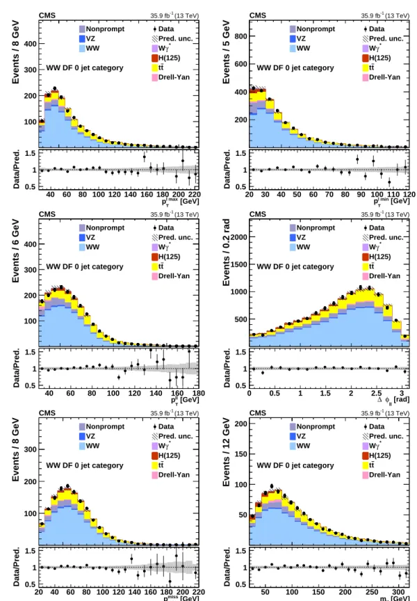
Table 1 summarizes the event selection criteria and Table 2 lists the sample composition after the fits described in Section 7 have been executed. Example kinematic distributions are shown in Fig. 1 for events with no jets and in Fig. 2 for events with exactly one jet. The simulations reproduce the observed distributions well.
5.2 Random forest selection
A random forest (RF) classifier is an aggregate of binary decision trees that have been trained independently and in parallel [11]. Each individual tree uses a random subset of features which mitigates against overfitting, a problem that challenges other classifiers based on decision trees. The random forest classifier is effective if there are many trees, and the aggregation of many trees averages out potential overfitting by individual trees. A random forest classifier is ex-pected to improve monotonically without overfitting [12] in contrast to other methods. Build-ing a random forest classifier requires less tunBuild-ing of hyperparameters compared, for example, with boosted decision trees, and its performance is as good [13].
The random forest analysis begins with a preselection that is close to the first set of require-ments in the sequential cut analysis. The selection of electrons and muons is identical. To avoid low-mass resonances and leptons from decays of hadrons, m`` > 30 GeV is required for both DF and SF events. To suppress the large background contribution from Z boson decays, events with SF leptons and with m`` within 15 GeV of the Z boson mass are rejected. Events with a third, loosely identified lepton with pT > 10 GeV are rejected to reduce backgrounds
50 100 150 200 [GeV] l max T p 0 100 200 300 400 Events / 8 GeV Data Pred. unc. * γ W H(125) t t Drell-Yan Nonprompt VZ WW WW DF 0 jet category (13 TeV) -1 35.9 fb CMS 40 60 80 100 120 140 160 180 200 220 [GeV] l max T p 0.5 1 1.5 Data/Pred. 20 40 60 80 100 120 [GeV] l min T p 0 200 400 600 800 Events / 5 GeV Data Pred. unc. * γ W H(125) t t Drell-Yan Nonprompt VZ WW WW DF 0 jet category (13 TeV) -1 35.9 fb CMS 20 30 40 50 60 70 80 90 100 110 120 [GeV] l min T p 0.5 1 1.5 Data/Pred. 50 100 150 [GeV] ll T p 0 100 200 300 400 Events / 6 GeV Data Pred. unc. * γ W H(125) t t Drell-Yan Nonprompt VZ WW WW DF 0 jet category (13 TeV) -1 35.9 fb CMS 40 60 80 100 120 140 160 180 [GeV] ll T p 0.5 1 1.5 Data/Pred. 0 1 2 3 [rad] ll φ ∆ 0 500 1000 1500 2000 Events / 0.2 rad Data Pred. unc. * γ W H(125) t t Drell-Yan Nonprompt VZ WW WW DF 0 jet category (13 TeV) -1 35.9 fb CMS 0 0.5 1 1.5 2 2.5 3 [rad] ll φ ∆ 0.5 1 1.5 Data/Pred. 50 100 150 200 [GeV] miss T p 0 100 200 300 Events / 8 GeV Data Pred. unc. * γ W H(125) t t Drell-Yan Nonprompt VZ WW WW DF 0 jet category (13 TeV) -1 35.9 fb CMS 20 40 60 80 100 120 140 160 180 200 220 [GeV] miss T p 0.5 1 1.5 Data/Pred. 100 200 300 [GeV] ll m 0 50 100 150 200 Events / 12 GeV Data Pred. unc. * γ W H(125) t t Drell-Yan Nonprompt VZ WW WW DF 0 jet category (13 TeV) -1 35.9 fb CMS 50 100 150 200 250 300 [GeV] ll m 0.5 1 1.5 Data/Pred.
Figure 1: Kinematic distributions for events with zero jets and DF leptons in the sequential cut analysis. The distributions show the leading and trailing lepton pT (p`Tmaxand p`Tmin), the dilepton transverse momentum p``T , the azimuthal angle between the two leptons ∆φ``, the missing transverse momentum pmissT , and the dilepton invariant mass m``. The error bars on the data points represent the statistical uncertainty of the data, and the hatched areas represent the combined systematic and statistical uncertainty of the predicted yield in each bin. The last bin includes the overflow.
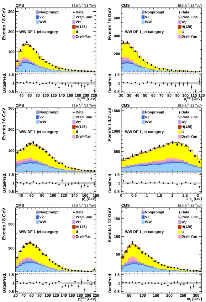
5.2 Random forest selection 7 50 100 150 200 [GeV] l max T p 0 100 200 300 Events / 8 GeV Data Pred. unc. * γ W H(125) t t Drell-Yan Nonprompt VZ WW WW DF 1 jet category (13 TeV) -1 35.9 fb CMS 40 60 80 100 120 140 160 180 200 220 [GeV] l max T p 0.5 1 1.5 Data/Pred. 20 40 60 80 100 120 [GeV] l min T p 0 200 400 600 Events / 5 GeV Data Pred. unc. * γ W H(125) t t Drell-Yan Nonprompt VZ WW WW DF 1 jet category (13 TeV) -1 35.9 fb CMS 20 30 40 50 60 70 80 90 100 110 120 [GeV] l min T p 0.5 1 1.5 Data/Pred. 50 100 150 [GeV] ll T p 0 100 200 300 Events / 6 GeV Data Pred. unc. * γ W H(125) t t Drell-Yan Nonprompt VZ WW WW DF 1 jet category (13 TeV) -1 35.9 fb CMS 40 60 80 100 120 140 160 180 [GeV] ll T p 0.5 1 1.5 Data/Pred. 0 1 2 3 [rad] ll φ ∆ 0 500 1000 1500 Events / 0.2 rad Data Pred. unc. * γ W H(125) t t Drell-Yan Nonprompt VZ WW WW DF 1 jet category (13 TeV) -1 35.9 fb CMS 0 0.5 1 1.5 2 2.5 3 [rad] ll φ ∆ 0.5 1 1.5 Data/Pred. 50 100 150 200 [GeV] miss T p 0 100 200 Events / 8 GeV Data Pred. unc. * γ W H(125) t t Drell-Yan Nonprompt VZ WW WW DF 1 jet category (13 TeV) -1 35.9 fb CMS 20 40 60 80 100 120 140 160 180 200 220 [GeV] miss T p 0.5 1 1.5 Data/Pred. 100 200 300 [GeV] ll m 0 50 100 150 Events / 12 GeV Data Pred. unc. * γ W H(125) t t Drell-Yan Nonprompt VZ WW WW DF 1 jet category (13 TeV) -1 35.9 fb CMS 50 100 150 200 250 300 [GeV] ll m 0.5 1 1.5 Data/Pred.
Figure 2: Kinematic distributions for events with exactly one jet and DF leptons in the sequen-tial cut analysis. The quantities, error bars, and hatched areas are the same as in Fig. 1.
Table 1: Summary of the event selection criteria for the sequential cut and the random forest analyses. DYMVA refers to an event classifier used in the sequential cut analysis to suppress Drell–Yan background events. RF refers to random forest classifiers. Kinematic quantities are measured in GeV. The symbol (—) means no requirement applied.
Quantity Sequential Cut Random Forest
DF SF DF SF
Number of leptons Strictly 2 Strictly 2
Lepton charges Opposite Opposite
p`Tmax >25 >25 p`Tmin >20 >20 m`` >20 >40 >30 >30 Additional leptons 0 0 |m``−mZ| — >15 — >15 p``T >30 >30 — — pmissT >20 >55 — —
pmiss,projT , pmiss,track projT >20 >20 — —
Number of jets ≤1 — —
Number of b-tagged jets 0 0
DYMVA score — >0.9 — —
Drell–Yan RF score SDY — — >0.96
tt RF score Stt — — >0.6
from VZ production. Finally, events with one or more b-tagged jets (pbT >20 GeV and medium working point) are rejected, since the background from tt production is characterized by the presence of b jets whereas the signal is not. These requirements are known as the preselection requirements.
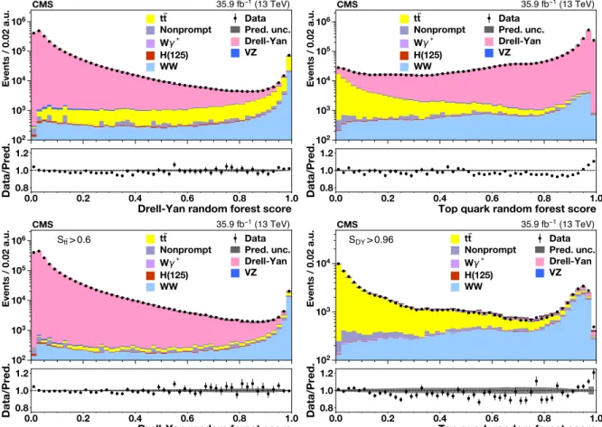
After the preselection, the largest background contamination comes from Drell–Yan produc-tion of lepton pairs and tt producproduc-tion with both top quarks producing prompt leptons. To reduce these backgrounds, two independent random forest classifiers are constructed: an anti-Drell–Yan classifier optimized to distinguish anti-Drell–Yan and W+W−signal events, and an anti-tt classifier optimized to distinguish anti-tt and W+W−events. The classifiers produce scores, SDY and Stt, arranged so that signal appears mainly at SDY ≈ 1 and Stt ≈ 1 while backgrounds appear mainly at SDY ≈ 0 and Stt ≈ 0. Figure 3 shows the distributions of the scores for the two random forest classifiers. The signal region is defined by the requirements SDY >SminDY and Stt > Smintt . For the cross section measurement, the specific values SminDY = 0.96 and Sttmin = 0.6 are set by simultaneously minimizing the uncertainty in the cross section and maximizing the purity of the selected sample. For measuring the jet multiplicity, a lower value of Smin
tt = 0.2
is used, which increases the efficiency for W+W−events with jets. A Drell–Yan control region is defined by SDY < 0.6 and Stt > 0.6 and a tt control region is defined by SDY > 0.6 and Stt <0.6. The event selection used in this measurement is summarized in Table 1.
The architecture of the two random forest classifiers is determined through an optimization of hyperparameters explored in a grid-like fashion. The optimal architecture for this problem has 50 trees with a maximum tree depth of 20; the minimum number of samples per split is 50 and the minimum number of samples for a leaf is one. The maximum number of features seen by any single tree is the square-root of the total number of features (ten for the DY random forest and eight for the tt random forest).
9
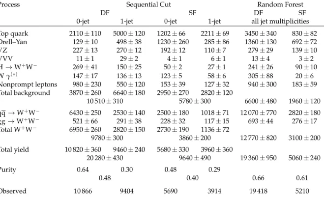
Table 2: Sample composition for the sequential cut and random forest selections after the fits described in Section 7 have been executed; the uncertainties shown are based on the total un-certainty obtained from the fit. The purity is the fraction of selected events that are W+W− signal events. “Observed” refers to the number of events observed in the data.
Process Sequential Cut Random Forest
DF SF DF SF
0-jet 1-jet 0-jet 1-jet all jet multiplicities
Top quark 2110±110 5000±120 1202±66 2211±69 3450±340 830±82 Drell–Yan 129±10 498±38 1230±260 285±86 1360±130 692±72 VZ 227±13 270±12 192±12 110±7 279±29 139±10 VVV 11±1 29±2 4±1 6±1 13±4 3±2 H→W+W− 269±41 150±25 50±2 27±1 241±26 90±10 W γ(∗) 147±17 136±13 123±5 58±6 305±88 20±6 Nonprompt leptons 980±230 550±120 153±39 127±32 940±300 183±59 Total background 3870±260 6640±180 2950±270 2820±120 10 510±310 5780±300 6600±480 1960±120 qq →W+W− 6430±250 2530±140 2500±180 1018±71 12 070±770 2820±180 gg→W+W− 521±66 291±38 228±32 117±15 693±44 276±17 Total W+W− 6950±260 2820±150 2730±190 1136±72 9780±300 3860±200 12 770±820 3100±200 Total yield 10 820±360 9460±240 5680±330 3960±360 20 280±430 9640±490 19 360±950 5060±240 Purity 0.64 0.30 0.48 0.29 0.48 0.40 0.66 0.61 Observed 10 866 9404 5690 3914 19 418 5210
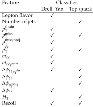
The random forest classifier takes as input some of the kinematic quantities listed in Table 1 and several other event features as listed in Table 3. These include the invariant mass of the two leptons and the missing momentum vector m``pmiss
T , the azimuthal angle between the lepton
pair and the missing momentum vector∆φ``pmiss
T , the smallest azimuthal angle between either
lepton and any reconstructed jet ∆φ`J, and the smallest azimuthal angle between the missing
momentum vector and any jet ∆φpmiss
T J. The random forest classifier also makes use of the
scalar sum of jet transverse momenta HT, and of the vector sum of the jet transverse momenta, referred to as the recoil in the event.
The sample composition for the signal region is summarized in Table 2. The signal efficiency and purity are higher than in the sequential cut analysis.
6
Background estimation
A combination of methods based on data control samples and simulations are used to estimate background contributions. The methods used in the sequential cut analysis and the random forest analysis are similar. The differences are described below.
The largest background contribution comes from tt and single top production which together are referred to as top quark production. This contribution arises when b jets are not tagged either because they fall outside the kinematic region where tagging is possible or because they receive low scores from the CSVv2 b tagging algorithm. The sequential cut analysis defines a control region by requiring at least one b-tagged jet. The normalization of the top quark background in the signal region is set according to the number of events in this control region.
102 103 104 105 106 Events / 0.02 a.u. tt Nonprompt W * H(125) WW Data Pred. unc. Drell-Yan VZ 0.0 0.2 0.4 0.6 0.8 1.0
Drell-Yan random forest score
0.8 1.0 1.2 Data/Pred. CMS 35.9 fb1 (13 TeV) 102 103 104 105 106 Events / 0.02 a.u. tt Nonprompt W * H(125) WW Data Pred. unc. Drell-Yan VZ 0.0 0.2 0.4 0.6 0.8 1.0
Top quark random forest score
0.8 1.0 1.2 Data/Pred. CMS 35.9 fb1 (13 TeV) 102 103 104 105 106 Events / 0.02 a.u. tt Nonprompt W * H(125) WW Data Pred. unc. Drell-Yan VZ 0.0 0.2 0.4 0.6 0.8 1.0
Drell-Yan random forest score
0.8 1.0 1.2 Data/Pred. Stt> 0.6 CMS 35.9 fb1 (13 TeV) 102 103 104 Events / 0.02 a.u. tt Nonprompt W * H(125) WW Data Pred. unc. Drell-Yan VZ 0.0 0.2 0.4 0.6 0.8 1.0
Top quark random forest score
0.8 1.0 1.2 Data/Pred. SDY> 0.96 CMS 35.9 fb1 (13 TeV)
Figure 3: Top left: score SDY distribution for the Drell–Yan discriminating random forest dis-criminant. The Drell–Yan distribution peaks toward zero and the W+W− distribution peaks toward one. Top right: score Stt distribution for the top quark random forest discriminant. The tt distribution peaks toward zero and the W+W−peaks toward one. Bottom left: the SDY distribution after suppressing top quark events with Stt > Smintt = 0.6. Bottom right: the Stt distribution after suppressing Drell–Yan events with SDY > SminDY = 0.96. The error bars on the points represent the statistical uncertainties for the data, and the hatched areas represent the combined systematic and statistical uncertainties of the predicted yield in each bin.
11
Table 3: Features used for the random forest classifiers. The first classifier distinguishes Drell– Yan and W+W−signal events, and the second one distinguishes top quark events and signal events.
Feature Classifier
Drell–Yan Top quark
Lepton flavor X Number of jets X p`Tmin X pmissT X X pmiss,projT X p``T X X m`` X m``pmiss T X ∆φ``pmissT X X ∆φ`J X ∆φpmiss T J X ∆φ`` X HT X Recoil X X
Similarly, the random forest analysis defines a top quark control region on the basis of scores: SDY > 0.6 and Stt < 0.6. Many kinematic distributions are examined and all show good agreement between simulation and data in this control region. This control region is used to set the normalization of the top quark background in the signal region.
The next largest background contribution comes from the Drell–Yan process, which is larger in the SF channel than in the DF channel. The nature of these contributions is somewhat different. The SF contribution arises mainly from the portion of Drell–Yan production that falls below or above the Z resonance peak. The sequential analysis calibrates this contribution using the ob-served number of events in the Z peak and the ratio of numbers of events inside and outside the peak, as estimated from simulations. The DF contribution arises from Z → τ+τ− production with both τ leptons decaying leptonically. The sequential cut analysis verifies the Z → τ+τ− background using a control region defined by meµ < 80 GeV and inverted p``T requirements. The random forest analysis defines a Drell–Yan control region by SDY < 0.6 and Stt > 0.6, which includes both SF and DF events. Simulations of kinematic distributions for events in this region match the data well, and the yield of events in this region is used to normalize the Drell–Yan background contribution in the signal region.
The next most important background contribution comes mainly from W boson events in which a nonprompt lepton from a jet is selected in addition to a lepton from the W boson decay. Monte Carlo simulation cannot be used for an accurate estimate of this contribution, but it can be used to devise and evaluate an estimate based on control samples. In the sequential cut analysis, a “pass-fail” control sample is defined by one lepton that passes the lepton selection criteria and another that fails the criteria but passes looser criteria. The misidentification rate f for a jet that satisfies loose lepton requirements to also pass the standard lepton requirements is determined using an event sample dominated by multijet events with nonprompt leptons. This misidentification rate is parameterized as a function of lepton pT and η and used to com-pute weights f /(1− f)in the pass-fail sample that are used to determine the contribution of nonprompt leptons in the signal region [46, 47]. The random forest analysis uses a different
method based on a control region in which the two leptons have the same charge. This control region is dominated by W+jets events with contributions from diboson and other events. The transfer factor relating the number of same-sign events in the control region to the number of opposite-sign events in the signal region is based on two methods relying on data control sam-ples and which are validated using simulations. One method uses events with DF leptons and low pmissT and the other uses events with an inverted isolation requirement. Both methods yield values for the transfer factor that are consistent at the 16% level.
Background contamination from Wγ∗events with low-mass γ∗ → `+`−can satisfy the signal event selection when the transverse momenta of the two leptons are very different [46]. The predicted contribution in the signal region is normalized to the number of events in a control region with three muons satisfying pT >10, 5, and 3 GeV and for mγ∗ <4 GeV. In this control region, the requirement pmissT < 25 GeV is imposed in order to suppress non-Wγ∗events. The remaining minor sources of background, including diboson and triboson final states and Higgs-mediated W+W− production, are evaluated using simulations normalized to the most precise theoretical cross sections available.
7
Signal extraction
The cross sections are obtained by simultaneously fitting the predicted yields to the observed yields in the signal and control regions. In this fit, a signal strength parameter modifies the predicted signal yield defined by the central value of the theoretical cross section, σtotNNLO = 118.8±3.6 pb. The fitted value of the signal strength is expected to be close to unity if the SM is valid, and the measured cross section is the product of the signal strength and the theo-retical cross section. Information from control regions is incorporated in the analysis through additional parameters that are free in the fit; the predicted background in the signal region is thereby tied to the yields in the control regions. In the sequential cut analysis, there is one control region enriched in tt events; the yields in the signal and this one control region are fit simultaneously. Since the selected event sample is separated according to SF and DF, 0- and 1-jet selections, there are eight fitted yields. In the random forest analysis there are three control regions, one for Drell–Yan background, a second for tt background, and a third for events with nonprompt leptons (e.g., W+jets). Since SF and DF final states are analyzed together, and the selection does not explicitly distinguish the number of jets, there are four fitted yields in the random forest analysis. In both analyses, the yields in the control regions effectively constrain the predicted backgrounds in the signal regions.
Additional nuisance parameters are introduced in the fit that encapsulate important sources of systematic uncertainty, including the electron and muon efficiencies, b tagging efficiencies, the jet energy scale, and the predicted individual contributions to the background. The total signal strength uncertainty, including all systematic uncertainties, is determined by the fit with all parameters free; the statistical uncertainty is determined by fixing all parameters except the signal strength to their optimal values.
8
Systematic uncertainties
Experimental and theoretical sources of systematic uncertainty are described in this section. A summary of all systematic uncertainties for the cross section measurement is given in Table 4. These sources of uncertainty impact the measurements of the cross section through the normal-ization of the signal. Many of them also impact kinematic distributions that ultimately can alter
8.1 Experimental sources of uncertainty 13
the shapes of distributions studied in this analysis. Both normalization and shape uncertainties are evaluated.
8.1 Experimental sources of uncertainty
There are several sources of experimental systematic uncertainties, including the lepton effi-ciencies, the b-tagging efficiency for b quark jets and the mistag rate for light-flavor quark and gluon jets, the lepton momentum and energy scales, the jet energy scale and resolution, the modeling of pmissT and of pileup in the simulation, the background contributions, and the integrated luminosity.
The sequential cut and the random forest analyses both use control regions to estimate the background contributions in the signal region. The uncertainties in the estimates are deter-mined mainly by the statistical power of the control regions, though the uncertainty of the theoretical cross sections and the shape of the Z resonant peak also play a role. Sources of sys-tematic uncertainty of the estimated Drell–Yan background include the Z resonance line shape and the performance of the DYMVA classifier for different pmissT thresholds. These uncertain-ties are propagated directly to the predicted SF and DF background estimates. The contribution from nonprompt leptons is entirely determined by the methods based on data control regions, described in Section 6; typically these contributions are uncertain at approximately the 30% level. The contribution from the Wγ∗final state is checked using a sample of events with three well-identified leptons including a low-mass, opposite-sign pair of muons. The comparison of the MC prediction with the data has an uncertainty of about 20%. The other backgrounds are estimated using simulations and their uncertainties depend on the uncertainties of the theo-retical cross sections, which are typically below 10%. Statistical uncertainties from the limited number of MC events are taken into account, and have a very small impact on the result. Small differences in the lepton trigger, reconstruction, and identification efficiencies for data and simulation are corrected by applying scale factors to adjust the efficiencies in the simu-lation. These scale factors are obtained using events in the Z resonance peak region [42, 43] recorded with unbiased triggers. They vary with lepton pT and η and are within 3% of unity. The uncertainties of these scale factors are mostly at the 1–2% level.
Differences in the probabilities for b jets and light-flavor quark and gluon jets to be tagged by theCSVv2 algorithm are corrected by applying scale factors to the simulation. These scale factors are measured using tt events with two leptons [40]. These scale factors are uncertain at the percent level and have relatively little impact on the result because the signal includes mainly light-flavor quark and gluon jets, which have a low probability to be tagged, and the top quark background is assessed using appropriate control regions.
The jet energy scale is set using a variety of in situ calibration techniques [48]. The remaining uncertainty is assessed as a function of jet pT and η. The jet energy resolution in simulated events is slightly different than that measured in data. The differences between simulation and data lead to uncertainties in the efficiency of the event selection because the number of selected jets, their transverse momenta, and also pmissT play a role in the event selection.
The lepton energy scales are set using the position of the Z resonance peak; the uncertainties are very small and have a negligible impact on the measurements reported here.
The modeling of pileup depends on the total inelastic pp cross section [49]. The pileup uncer-tainty is evaluated by varying this cross section up and down by 5%.
lead to a systematic uncertainty from the background predictions. It is listed as part of the experimental systematic uncertainty in Table 4.
The uncertainty in the integrated luminosity measurement is 2.5% [50]. It contributes directly to the cross section and also to the uncertainty in the minor backgrounds predicted from simu-lation.
8.2 Theoretical sources of uncertainty
The efficiency of the event selection is sensitive to the number of hadronic jets in the event. The sequential cut analysis explicitly singles out events with zero or one jet, and the random forest classifiers utilize quantities, such as HT, that tend to correlate with the number of jets. As a consequence, the efficiency of the event selection is sensitive to higher-order QCD corrections that are adequately described by neither the matrix-element calculation ofPOWHEGnor by the
parton shower simulation. The uncertainty reflecting these missing higher orders is evaluated by varying the QCD factorization and renormalization scales independently up and down by a factor of two but excluding cases in which one is increased and the other decreased simulta-neously. A change in measured cross sections is evaluated by applying appropriate weights to the simulated events.
Some of the higher-order QCD contributions to W+W−production have been calculated using the pT-resummation [51, 52] and the jet-veto resummation [53] techniques. The results from these two approaches are compatible [54]. The transverse momentum pWWT of the W+W− pair is used as a proxy for these higher-order corrections; the pWWT spectrum from POWHEG
is reweighted to match the analytical prediction obtained using the pT-resummation at next-to-next-to-leading logarithmic accuracy [51]. Uncertainties in the theoretical calculation of the pWWT spectrum lead to uncertainties in the event selection efficiency that are assessed for the qq → W+W−process by independently varying the resummation, the factorization, and the renormalization scales in the analytical calculation [52]. The uncertainty in the gg → W+W− component is determined by the variation of the renormalization and factorization scales in the theoretical calculation of this process [9].
Additional sources of theoretical uncertainties come from the PDFs and the assumed value of αS. The PDF uncertainties are estimated, following the PDF4LHC recommendations [55], from the variance of the values obtained using the set of MC replicas of the NNPDF3.0 PDF set. The variation of both the signal and the backgrounds with each PDF set and the value of αS is taken into account.
The uncertainty from the modeling of the underlying event is estimated by comparing the signal efficiency obtained with the qq → W+W−sample described in Section 3 to alternative samples that use different generator configurations.
The branching fraction for leptonic decays of W bosons is taken to beB(W → `ν) =0.1086± 0.0009 [56], and lepton universality is assumed to hold. The uncertainty coming from this branching fraction is not included in the total uncertainty; it would amount to 1.8% of the cross section value.
9
The W
+W
−cross section measurements
Two measurements of the total production cross section are reported in this section: the pri-mary one coming from the sequential cut analysis and a secondary measurement coming from the random forest analysis. In addition, measurements of the fiducial cross section are
re-9.1 Total production cross section 15
Table 4: Relative systematic uncertainties in the total cross section measurement (0- and 1-jet, DF and SF) based on the sequential cut analysis.
Uncertainty source (%)
Statistical 1.2
tt normalization 2.0
Drell–Yan normalization 1.4
Wγ∗normalization 0.4
Nonprompt leptons normalization 1.9
Lepton efficiencies 2.1
b tagging (b/c) 0.4
Mistag rate (q/g) 1.0
Jet energy scale and resolution 2.3
Pileup 0.4
Simulation and data control regions sample size 1.0
Total experimental systematic 4.6
QCD factorization and renormalization scales 0.4 Higher-order QCD corrections and pWWT distribution 1.4
PDF and αS 0.4
Underlying event modeling 0.5
Total theoretical systematic 1.6
Integrated luminosity 2.7
Total 5.7
ported, based on the sequential cut analysis, including the change of the zero-jet cross section with variations of the jet pTthreshold.
9.1 Total production cross section
Both the sequential cut and random forest analyses provide precise measurements of the total production cross section. Since the techniques for selecting signal events are rather different, both values are reported here. The measurement obtained with the sequential cut analysis is the primary measurement of the total production cross section because it is relatively insensitive to the uncertainties in the corrections applied to the pWWT spectrum. The overlap of the two sets of selected events is approximately 50%. A combination of the two measurements is not carried out because the reduction in the uncertainty would be minor.
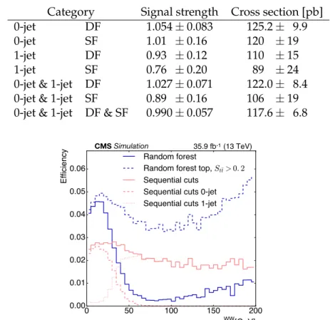
The sequential cut (SC) analysis makes a double-dichotomy of the data: selected events are separated if the leptons are DF or SF (DF is purer because of a smaller Drell-Yan contamination), and these are further subdivided depending on whether there is zero or one jet (0-jet is purer because of a smaller top quark contamination). The comparison of the four signal strengths provides an important test of the consistency of the measurement; the cross section value is based on the simultaneous fit of DF & SF and 0-jet & 1-jet channels. The result is σSCtot =117.6± 1.4 (stat)±5.5 (syst)±1.9 (theo)±3.2 (lumi) pb = 117.6±6.8 pb, which is consistent with the theoretical prediction σtotNNLO = 118.8±3.6 pb. A summary of the measured signal strengths and the corresponding cross sections is given in Table 5.
The random forest analysis isolates a purer signal than the sequential cut analysis (see Ta-ble 2); however, its sensitivity is concentrated at relatively low pWWT as shown in Fig. 4. This
Table 5: Summary of the signal strength and total production cross section obtained in the sequential cut analysis. The uncertainty listed is the total uncertainty obtained from the fit to the yields.
Category Signal strength Cross section [pb]
0-jet DF 1.054±0.083 125.2± 9.9
0-jet SF 1.01 ±0.16 120 ±19
1-jet DF 0.93 ±0.12 110 ±15
1-jet SF 0.76 ±0.20 89 ±24
0-jet & 1-jet DF 1.027±0.071 122.0± 8.4
0-jet & 1-jet SF 0.89 ±0.16 106 ±19
0-jet & 1-jet DF & SF 0.990±0.057 117.6± 6.8
0 50 100 150 200 pWW T [GeV] 0.00 0.01 0.02 0.03 0.04 0.05 0.06 Efficiency Random forest
Random forest top, St¯t>0.2
Sequential cuts Sequential cuts 0-jet Sequential cuts 1-jet
CMSSimulation 35.9 fb-1 (13 TeV)
Figure 4: Comparison of efficiencies for the sequential cut and random forest analyses as a function of pWWT . The sequential cut analysis includes 0- and 1-jet events from both DF and SF lepton combinations, for which the contributions from 0- and 1-jet are shown separately. The efficiency curve for Smin
tt =0.2 is also shown; this value is used in measuring the jet multiplicity
distribution.
region corresponds mainly to events with zero jets; the random forest classifier uses observ-ables such as HT that correlate with jet multiplicity and reduce top quark background con-tamination by favoring events with a low jet multiplicity. As a consequence, the random forest result is more sensitive to uncertainties in the theoretical corrections to the pWWT spec-trum than the sequential cut analysis. The signal strength measured by the random forest analysis is 1.106±0.073 which corresponds to a measured total production cross section of σRFtot = 131.4±1.3 (stat)±6.0 (syst)±5.1 (theo)±3.5 (lumi) pb= 131.4±8.7 pb. The difference with respect to the sequential cut analysis reflects the sensitivity of the random forest analysis to low pWWT .
9.2 Fiducial cross sections
The sequential cut analysis is used to obtain fiducial cross sections. The definition of the fiducial region is similar to the requirements described in Section 5.1 above. The generated event record must contain two prompt leptons (electrons or muons) with pT >20 GeV and|η| <2.5. Decay products of τ leptons are not considered part of the signal in this definition of the fiducial region. Other kinematic requirements are applied: m`` > 20 GeV, p``T > 30 GeV, and pmissT >
17
20 GeV (where pmissT is calculated using the momenta of the neutrinos emitted in the W boson decays). When categorizing events with zero or more jets, a jet is defined using stable particles but not neutrinos. For the baseline measurements, the jets must have pT >30 GeV and|η| <4.5 and be separated from each of the two leptons by∆R>0.4.
The fiducial cross section is obtained by means of a simultaneous fit to the DF and SF, 0- and 1-jet final states. The measured value is σfid=1.529±0.020 (stat)±0.069 (syst)±0.028 (theo)± 0.041 (lumi) pb = 1.529±0.087 pb, which agrees well with the theoretical value σNNLOfid = 1.531±0.043 pb. These values are corrected to the fiducial region with all jet multiplicities. The fiducial cross sections for the production of W+W−boson pairs with zero or one jet are of interest because some of the earlier measurements were based on the 0-jet subset only, i.e., a jet veto was applied [2–4, 6]. The sequential cut analysis provides the following values based on the combination of the DF and SF categories: σfid(0-jet) = 1.61±0.10 pb and σfid(1-jet) = 1.35±0.11 pb for a jet pTthreshold of 30 GeV. These fiducial cross section values pertain to the definition given above, in particular, they pertain to all jet multiplicities.
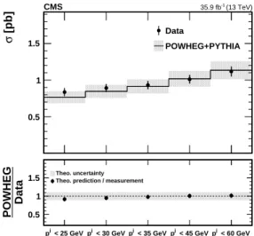
The fiducial cross section for W+W−+0-jets production is also measured as a function of the jet pTthreshold in the range 25–60 GeV with the results listed in Table 6 and displayed in Fig. 5. The cross section is expected to increase with jet pTthreshold because the phase space for zero jets increases.
Table 6: Fiducial cross section for the production of W+W−+0-jets as the pT threshold for jets is varied. The fiducial region is defined by two opposite-sign leptons with pT > 20 GeV and|η| <2.5 excluding the products of τ lepton decay, and m`` > 20 GeV, p``T > 30 GeV, and
pmiss
T >30 GeV. Jets must have pTabove the stated threshold,|η| <4.5, and be separated from
each of the two leptons by∆R>0.4. The total uncertainty is reported. pTthreshold (GeV) Signal strength Cross section (pb)
25 1.091±0.073 0.836±0.056
30 1.054±0.065 0.892±0.055
35 1.020±0.060 0.932±0.055
45 0.993±0.057 1.011±0.058
60 0.985±0.059 1.118±0.067
10
Normalized differential cross section measurements
Differential cross sections are measured for the fiducial region defined above using the sequential-cut, DF event selection. The random forest selection is unsuitable for measuring these differen-tial cross sections because some of these kinematic quantities are used as inputs to the random forest classifiers. These differential cross sections are normalized to the measured integrated fiducial cross section, which for the DF final state (0- and 1-jet) is 0.782±0.053 pb corresponding to a signal strength of 1.022±0.069.
For each differential cross section, a simultaneous fit to the reconstructed distribution is per-formed in the following manner. An independent signal strength parameter is assigned to each level histogram bin. For the MC simulated events falling within a given generator-level bin, a template histogram of the reconstructed kinematic quantity is formed. The de-tector resolution is good for the quantities considered, so the template histogram has a peak corresponding to the given generator-level bin; the contents of all bins below and above the given generator-level bin are relatively low. When the fit is performed, the signal strengths are
< 25 GeV j T p j < 30 GeV T p j < 35 GeV T p j < 45 GeV T p j < 60 GeV T p [pb] σ 0 0.5 1 1.5 Data POWHEG+PYTHIA (13 TeV) -1 35.9 fb CMS < 25 GeV j T p j < 30 GeV T p j < 35 GeV T p j < 45 GeV T p j < 60 GeV T p Data POWHEG 0.5 1
1.5 Theo. uncertaintyTheo. prediction / measurement
Figure 5: The upper panel shows the fiducial cross sections for the production of W+W−+ 0-jets as the pT threshold for jets is varied. The fiducial region is defined by two opposite-sign leptons with pT > 20 GeV and|η| < 2.5 excluding the products of τ lepton decay, and m`` > 20 GeV, p``T > 30 GeV, and pmissT > 30 GeV. Jets must have pT above the stated threshold, |η| <4.5, and be separated from each of the two leptons by∆R> 0.4. The lower panel shows the ratio of the theoretical prediction to the measurement. In both the upper and lower panels, the error bars on the data points represent the total uncertainty of the measurement, and the shaded band depicts the uncertainty of the MC prediction.
allowed to vary independently. The correlations among bins in the distribution of the recon-structed quantity are taken into account. The fitted values of the signal strength parameters are applied to the generator-level differential cross section to obtain the measured differential cross section.
Measurements of the differential cross sections with respect to the dilepton mass(1/σ)dσ/dm``, the leading lepton transverse momentum(1/σ)dσ/dp`Tmax, the trailing lepton transverse mo-mentum(1/σ)dσ/dp`Tmin, and the angular separation between the leptons(1/σ)dσ/d∆φ``are reported. The measurements are compared to simulations generated withPOWHEG+PYTHIAin
Fig. 6.
11
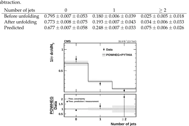
Jet multiplicity measurement
A measurement of the jet multiplicity tests the accuracy of theoretical calculations and event generators. Signal W+W− events are characterized by a low jet multiplicity in contrast to tt background events, which typically have two or three jets. The sequential event selection ex-ploits this difference by eliminating events with more than one jet and by separating 0- and 1-jet event categories. The random forest selection, in contrast, places no explicit requirements on the number of jets (NJ) in an event, and the separation of signal W+W−events and tt back-ground utilizes other event features listed in Table 3. As a consequence, a precise measurement of the fractions of events with NJ = 0, 1, or ≥ 2 jets can be made. For this measurement, jets have pT > 30 GeV and|η| < 2.4, and must be separated from each of the selected leptons by ∆R >0.4. The rejection of events with one or more b-tagged jets is still in effect; however, the impact on the signal is very small.
19 [GeV] ll m 2 10 3 10 [1/bin]ll /dm σ d σ 1/ 0 0.1 0.2 Data POWHEG+PYTHIA (13 TeV) -1 35.9 fb CMS [GeV] ll m 2 10 103 Data POWHEG 0.5 1
1.5 Theo. uncertaintyTheo. prediction / measurement
[GeV] l max T p 2 10 [1/bin] max T /dp σ d σ 1/ 0 0.1 0.2 0.3 Data POWHEG+PYTHIA (13 TeV) -1 35.9 fb CMS [GeV] l max T p 2 10 Data POWHEG 0.5 1
1.5 Theo. uncertaintyTheo. prediction / measurement
2 10 [GeV] l min T p 0 0.1 0.2 0.3 0.4 [1/bin] min T /dp σ d σ 1/ Data POWHEG+PYTHIA (13 TeV) -1 35.9 fb CMS 2 10 [GeV] l min T p 0.5 1 1.5 Data POWHEG Theo. uncertainty Theo. prediction / measurement
[rad] ll φ ∆ 0 1 2 3 [1/bin] ll φ∆ /d σ d σ 1/ 0 0.1 0.2 0.3 Data POWHEG+PYTHIA (13 TeV) -1 35.9 fb CMS [rad] ll φ ∆ 0 1 2 3 Data POWHEG 0.5 1
1.5 Theo. uncertaintyTheo. prediction / measurement
Figure 6: The upper panels show the normalized differential cross sections with respect to the dilepton mass m``, leading lepton p`Tmax, trailing lepton p
`min
T , and dilepton azimuthal angular
separation ∆φ``, compared to POWHEG predictions. The lower panels show the ratio of the theoretical predictions to the measured values. The meaning of the error bars and the shaded bands is the same as in Fig. 5.
The anti-tt random forest produces a continuous score, Stt, in the range 0 ≤ Stt ≤ 1, as ex-plained in Section 5.2. For the measurement of the jet multiplicity presented in this section, the criterion against tt background is loosened to Smintt = 0.2 while SminDY = 0.96 remains. This looser requirement leads to a signal efficiency for the random forest selection with a relatively gentle variation with NJas shown in Table 7, and also a more even variation of the efficiency as a function of pWWT , as shown in Fig. 4. These efficiencies are defined for the events passing the random forest selection with respect to those passing the preselection requirements. The efficiency for the preselection is essentially independent of NJ.
Table 7: Efficiency for the random forest selection with respect to preselected events as a func-tion of jet multiplicity. The stated uncertainties are statistical only.
Number of jets 0 1 ≥2
Efficiency 0.555±0.003 0.448±0.004 0.290±0.004
Background contributions are subtracted from the observed numbers of events as a function of NJand then corrections are applied for the random forest efficiencies shown in Table 7. The observed jet multiplicity suffers from the migration of events from one NJ bin to another due to two experimental effects: first, pileup can produce extra jets (pileup), and second, jet energy mismeasurements can lead to jets with true pTbelow the 30 GeV threshold being accepted and others with true pTabove 30 GeV being rejected. Pileup jets only increase the number of jets in an event while energy calibration and resolution leads to both increases and decreases in NJ. Because of the falling jet pT distribution, the jet energy resolution leads to increases in NJmore often than to decreases.
The two sources of event migration are corrected in two distinct steps. The signal MC event sample is used to build two response matrices: RPU for pileup and Rdet for detector effects, in particular, jet energy resolution. The reconstructed jet multiplicity for the signal process is given by~v = RPURdet~t where~v and~t are vectors representing the multiplicity distribution; ~t represents the MC “truth” as inferred from generator-level jets and~v is the reconstructed distribution. Generator-level jets are reconstructed from generated stable particles, excluding neutrinos, with the clustering algorithm used to reconstruct jets in data. These jets must satisfy pT > 30 GeV and|η| < 2.4 and must be separated by∆R > 0.4 from both of the two leptons from W boson decays. Reconstructed and generator-level jets are said to match if they have ∆R < 0.4. On the basis of the simulated signal event sample, the two response matrices are close to being diagonal:
RPU= 0.986 0 0 0.013 0.985 0 0.001 0.015 1 Rdet= 0.963 0.060 0.003 0.036 0.891 0.090 0.001 0.049 0.906 .
Here, the columns correspond to NJ = 0, 1, ≥ 2 for generator-level jets, and the rows to the same for reconstructed jets.
The response matrices are used to unfold the distribution of jet multiplicities according to~u=
RDET−1RPU−1~v. No regularization procedure is applied. The fractions of events with NJ = 0, 1,≥2 jets are obtained by normalizing~u to unit norm: the unfolded result is~w= ~u/|~u|. All systematic uncertainties are reevaluated for the jet multiplicity measurement. Since the
21
observables are essentially yields normalized to the total number of events, systematic un-certainties from the integrated luminosity and lepton efficiency are negligible. The statistical uncertainty in the response matrix is also negligible. Nonnegligible uncertainties are obtained for the jet energy scale and resolution, for pileup reweighting, and for reweighting of the pWWT spectrum. The total relative uncertainties for the elements of the response matrix are:
0.011 0.193 0.374 0.210 0.007 0.140 0.305 0.181 0.015 .
Although the relative uncertainty of the off-diagonal matrix elements is large, those elements themselves are small, so a precise measurement is still achievable.
Table 8 reports the measured fractions of events with NJjets. The fractions before unfolding for pileup and jet energy resolution are listed, as well as the prediction based onPOWHEGweighted to correct the W+W− pTspectrum. Figure 7 shows a comparison of the measured fractions and the prediction fromPOWHEG. For this prediction, the pWWT spectrum is reweighted as described in Section 8.2.
Table 8: Fractions of events with NJ =0, 1,≥ 2 jets. The first uncertainty is statistical and the second combines systematic uncertainties from the response matrix and from the background subtraction. Number of jets 0 1 ≥2 Before unfolding 0.795±0.007±0.053 0.180±0.006±0.039 0.025±0.005±0.018 After unfolding 0.773±0.008±0.075 0.193±0.007±0.043 0.034±0.006±0.033 Predicted 0.677±0.007±0.058 0.248±0.007±0.033 0.075±0.006±0.026 Number of jets 0 1 ≥ 2 J /dN σ d σ 1/ 0 0.5 1 Data POWHEG+PYTHIA (13 TeV) -1 35.9 fb CMS Number of jets 0 1 ≥ 2 Data POWHEG 0.5 1 1.5 2 Theo. uncertainty Theo. prediction / measurement
Figure 7: The upper panel shows the fractions of events with NJ = 0, 1, ≥ 2 jets. The filled circles represent the data after backgrounds are subtracted and pileup and energy resolution are taken into account. The solid lines represent the POWHEG+PYTHIAprediction. The lower panel shows the ratio of the theoretical prediction to the measurement. The meaning of the error bars and the shaded bands is the same as in Fig. 5.