A Hardware implementation of true-motion estimation with 3-D recursive search block matching algorithm

i

T.C

BAHÇEŞEHĐR ÜNĐVERSĐTESĐ

A HARDWARE IMPLEMENTATION OF

TRUE-MOTION ESTIMATION WITH 3-D RECURSIVE

SEARCH BLOCK MATCHING ALGORITHM

Master Thesis

SONER DEDEOĞLU

ii

T.C

BAHÇEŞEHĐR ÜNĐVERSĐTESĐ

A HARDWARE IMPLEMENTATION OF

TRUE-MOTION ESTIMATION WITH 3-D RECURSIVE

SEARCH BLOCK MATCHING ALGORITHM

Master Thesis

SONER DEDEOĞLU

Supervisor: ASST. PROF. DR. HASAN FATĐH UĞURDAĞ

iii

T.C

BAHÇEŞEHĐR ÜNĐVERSĐTESĐ INSTITUTE OF SCIENCE COMPUTER ENGINEERING

Name of the thesis: A Hardware Implementation of True-Motion Estimation with 3-D Recursive Search Block Matching Algorithm

Name/Last Name of the Student: Soner DEDEOĞLU Date of Thesis Defense: 30 January 2008

The thesis has been approved by the Institute of Science.

Assoc. Prof. Dr. Đrini DĐMĐTRĐYADĐS

Director

___________________

I certify that this thesis meets all the requirements as a thesis for the degree of Master of Science.

Asst. Prof. Dr. Adem KARAHOCA Program Coordinator

____________________

This is to certify that we have read this thesis and that we find it fully adequate in scope, quality and content, as a thesis for the degree of Master of Science.

Examining Committee Members Signature

Asst. Prof. Dr. Hasan Fatih UĞURDAĞ ____________________

Prof. Dr. Ali GÜNGÖR ____________________

Prof. Dr. Nizamettin AYDIN ____________________

Prof. Dr. Emin ANARIM ____________________

iv

ACKNOWLEDGMENTS

This thesis is dedicated to my family for their patience and understanding during my master’s study and the writing of this thesis. I am also grateful to Ahmet ÖZUĞURLU for his moral and spiritual support.

I would like to express my gratitude to Asst. Prof. Dr. Hasan Fatih UĞURDAĞ for not only being such a great supervisor but also encouraging and challenging me throughout my academic program.

I wish to thank Ali SAYINTA, Sinan YALÇIN, and Ümit MALKOÇ who provided me with great environment at Vestel – Vestek Research and Development Department during my thesis studies.

I also thank Prof. Dr. Şenay YALÇIN, Prof. Dr. Ali GÜNGÖR, Prof. Dr. Nizamettin

AYDIN, Prof. Dr. Emin ANARIM, and Asst. Prof. Dr. Sezer GÖREN UĞURDAĞ for

their help on various topics in the areas of digital chip design and digital video processing, for their advice and time.

v

ABSTRACT

A HARDWARE IMPLEMENTATION OF

TRUE-MOTION ESTIMATION WITH 3-D RECURSIVE SEARCH BLOCK MATCHING ALGORITHM

DEDEOĞLU, Soner

Computer Engineering

Supervisor: Asst. Prof. Dr. Hasan Fatih UĞURDAĞ

January 2008, 53 pages

Motion estimation, in video processing, is a technique for describing a frame in terms of translated blocks of another reference frame. This technique increases the ratio of video compression by the efficient use of redundancy information between frames. The Block Matching based motion estimation methods, based on dividing frames into blocks and calculating a motion vector for each block, are accepted as motion estimation standards in video encoding systems by international enterprises, such as MPEG, ATSC, DVB and ITU. In this thesis study, a hardware implementation of 3-D Recursive Search Block Matching Algorithm for the motion estimation levels, global and local motion estimations, is presented.

vi

ÖZET

ÜÇ BOYUTLU ÖZYĐNELĐ ARAMA BLOK UYUMLAMA ALGORĐTMASI ĐLE GERÇEK-HAREKET TAHMĐNĐNĐN

DONANIMSAL GERÇEKLEŞTĐRMESĐ

DEDEOĞLU, Soner

Bilgisayar Mühendisliği

Tez Danışmanı: Yrd. Doç. Dr. Hasan Fatih UĞURDAĞ

Ocak 2008, 53 Sayfa

Hareket tahmini, dijital video işlemede, bir çerçevenin başka bir referans çerçevenin bloklarının çevrilmesi cinsinden tanımlanması tekniğine verilen isimdir. Bu teknik, çerçeveler arası artıklık bilgilerinin daha verimli kullanılması ile video sıkıştırma oranları yükseltilmesini sağlamaktadır. Çerçeveleri bloklara bölerek her blok için bir hareket vektörü hesaplamaya dayanan Blok Uyumlama bazlı hareket tahmini yöntemleri MPEG, ATSC, DVB ve ITU gibi uluslararası kuruluşlar tarafından video kodlama sistemlerinde hareket tahmini standartları olarak kabul edilmiştir. Bu tez çalışmasında hareket tahmini aşamalarından olan global ve lokal hareket tahmini için Üç Boyutlu Özyineli Arama Blok Uyumlama Algoritması donanımsal olarak gerçekleştirilmesi sunulmuştur.

Anahtar Kelimeler: Dijital Video Đşleme, Hareket Tahmini, Çok Büyük Ölçekli Tümleşik

vii

TABLE OF CONTENTS

LIST OF TABLES……… ix

LIST OF FIGURES……….. x

LIST OF ABBREVIATIONS……….. xii

LIST OF SYMBOLS……… xiv

1. INTRODUCTION………... 1

2. MOTION ESTIMATION ALGORITHMS……… 2

2.1. GLOBAL MOTION COMPENSATION………. 2

2.2. BLOCK MOTION COMPENSATION……… 3

2.3. MOTION ESTIMATION……….. 4

2.3.1. Error Function for Block-Matching Algorithms……….. 6

2.3.2. Full Search (FS) Algorithm……… 6

2.3.3. Three Step Search (TSS) Algorithm ………. 7

2.3.4. Two Dimensional Logarithmic (TDL) Search Algorithm……… 7

2.3.5. Four Step Search (FSS) Algorithm………... 8

2.3.6. Orthogonal Search Algorithm (OSA)………... 10

2.4. 3-D RECURSIVE SEARCH BLOCK MATCHING ALGORITHM…… 10

2.4.1. 1-D Recursive Search………. 11

2.4.2. 2-D Recursive Search………. 12

2.4.3. 3-D Recursive Search………. 15

2.5. GLOBAL MOTION ESTIMATION TECHNIQUE……….. 17

3. MOTION ESTIMATION HARDWARE……….. 20

3.1. VIDEO FORMAT………. 20

3.2. HIGH-LEVEL ARCHITECTURE OF HARDWARE……….. 21

3.3. PACKING STRATEGY OF PIXELS………. 23

3.4. GLOBAL MOTION ESTIMATOR………. 24

3.4.1. GME Memory Structure……….... 25

3.4.2. GME Processing Element Array………... 28

3.4.3. GME Minimum SAD Comparator……… 31

3.5. MEDIAN VECTOR GENERATION………... 31

3.6. LOCAL MOTION ESTIMATOR……… 32

3.6.1. Motion Vector Array……….. 33

3.6.2. LME Memory Structure………. 35

3.6.3. LME Processing Element Array……… 37

3.6.4. Adder Tree………... 39

3.6.5. LME Minimum SAD Comparator………. 40

4. VERIFICATION STRATEGY AND TOOLS…...……….. 41

4.1. MOTION DLL CLASSES……….... 41

4.1.1. MemoryBlock………. 42

4.1.2. SearchBlock……… 43

viii 4.1.4. FrameGenerator………. 43 4.1.5. MotionVector……….. 44 4.1.6. MotionEstimation……… 44 4.1.7. GlobalMotionEstimation………. 44 4.1.8. RecursiveTrueMotionEstimation………... 45

4.2. GUI FOR TEST SOFTWARE……….. 45

5. CONCLUSION AND FUTURE WORK……… 48

REFERENCES………. 50

ix

LIST OF TABLES

Table 2.1 : TSS algorithm………..……… 7

Table 2.2 : TDL algorithm……….………... 7

Table 2.3 : FSS algorithm……….……… 8

Table 2.4 : OSA algorithm……….………... 10

Table 3.1 : Input frame sequence and storage into DDR……….. 20

Table 3.2 : Timeline representation of DDR access, ME, and generation of output video sequence……… 21

Table 3.3 : Address generator states………..……… 26

Table 3.4 : Address generation algorithm………. 26

Table 3.5 : Data flow to processing elements over input luminance ports…... 29

Table 3.6 : PEs vs. corresponding luminance ports……….. 30

Table 3.7 : Value of pointer k due to motion vector input………... 37

x

LIST OF FIGURES

Figure 2.1 : Relation between reference frame, current frame and motion

vector………... 5

Figure 2.2 : Types of frame prediction………... 5

Figure 2.3 : Illustration of selection of blocks for different cases is FSS…….. 9

Figure 2.4 : The bidirectional convergence (2-D C) principle………... 13

Figure 2.5 : Locations around the current block, from which the estimation result could be used as a spatial prediction vector……….. 14

Figure 2.6 : Location of the spatial predictions of estimators a and b with respect to the current block………. 15

Figure 2.7 : The relative positions of the spatial predictors Sa and Sb and the convergence accelerators Ta and Tb………. 16

Figure 2.8 : Position of the sample SWs to find MVglobal in the image plane.... 18

Figure 3.1 : Video sequence composed of repeated frames………... 20

Figure 3.2 : High-level block diagram motion estimator/compensator architecture……….. 22

Figure 3.3 : Packing strategy of pixels and DDR storage………... 24

Figure 3.4 : Global motion estimator block diagram……….. 24

Figure 3.5 : Memory structure of global motion estimator………. 25

Figure 3.6 : GME_MEMO data access timeline and address generation……... 27

Figure 3.7 : Structure of GME processing element………. 28

Figure 3.8 : GME PE array structure………... 30

Figure 3.9 : Structure of GME minimum SAD comparator……… 31

Figure 3.10 : Local motion estimator block diagram……… 32

Figure 3.11 : Structure of motion vector array………. 33

Figure 3.12 : Structure of updater………. 34

Figure 3.13 : Galois LFSR………. 34

Figure 3.14 : Memory structure for local motion estimator……….. 35

Figure 3.15 : Selection of correct luminance value………... 37

Figure 3.16 : LME PE array structure………... 38

Figure 3.17 : Structure of LME processing element………. 38

xi

Figure 3.19 : Structure of LME minimum SAD comparator……… 40

Figure 4.1 : Testbench environment……… 41

Figure 4.2 : Class Diagram of Motion DLL……… 42

Figure 4.3 : Main user form of motion estimation test software………. 45

Figure 4.4 : “Baskirt - Amusement Park” sequence is loaded………. 46

Figure 4.5 : Initial motion vectors calculated by FS algorithm………... 46

Figure 4.6 : Global motion vector on coordinate plane……….. 47

Figure 4.7 : Local motion vectors calculated by 3-D RS algorithm…………... 47

Figure 4.8 : Motion estimation over “Phaeton” sequence with 352×240 resolution……….... 47

xii

LIST OF ABBREVIATIONS

Advanced Television Systems Committee : ATSC

Bidirectional Convergence : 2-D C

Block Motion Compensation : BMC

Carry Save Adder : CSA

Carry Propagate Adder : CPA

Device Under Test : DUT

Digital Video Broadcasting : DVB

Dual Data Rate : DDR

Dynamically Linked Library : DLL

Extended Graphics Array : XGA

Four Step Search Algorithm : FSS

Frame Rate Conversion : FRS

Full Search : FS

Global Motion Estimation : GME

Graphical User Interface : GUI

High Definition : HD

International Telecommunications Union : ITU

Linear Feedback Shift Register : LFSR

Liquid Crystal Display : LCD

Local Motion Estimation : LME

Luminance-Chrominance Color Space : YUV

Motion Compensation : MC

Motion Estimation : ME

Motion Vector : MV

Moving Picture Experts Group : MPEG

One-At-a-Time Search Algorithm : OTS

Orthogonal Search Algorithm : OSA

Processing Element : PE

Random Access Memory : RAM

Recursive Search : RS

xiii

Search Window : SW

Sum of Absolute Differences : SAD

Three Step Search Algorithm : TSS

Two Dimensional Logarithmic Search Algorithm : TDL

xiv

LIST OF SYMBOLS

Candidate set of position X on ithframe : CSi

( )

Candidate vector : C(X,t)

DDR input data : DDR _in

DDR output data : DDR_out

Error function due to candidate vector, C(X,t), on the position X : l(C,X,t)

Global motion vector : MV_global

Input frame : _{F in}

Maximum motion displacement : w

Macroblock with upper most left pixel at the location (m,n) : MBri(m,n)

Macroblock of position X : B(X)

Output frame : F _out

Spatial distance : r

Spatial recursive vector : S_a(X,t)

Sum of absolute differences due to displacement ( vu, ) : SAD( vu, )

Temporal recursive vector : Ta(X,t)

Position on the block grid : X

Prediction vector of position X on ithframe : Di(X,t)

Update value : L

Update vector : U

1

1. INTRODUCTION

There have been two significant revolutions in television history. First was in 1954 when the first color TV signals were broadcasted. Nowadays, black-and-white TV signals are unavailable in the airwaves. Second of the revolutions is eventuated by digital TV signals, broadcasted at the end of 1998 first on the air. Analog TV signals have been started to be disappeared from the airwaves as black-and-white TV signals.

Digital TV is not just a provider of quality in video; it also enables many multimedia applications and services to be introduced. While digital video and digital TV technologies are developing rapidly, they triggered the academic researches on the subject, digital video processing. Video processing differs from image processing due to the movements of the objects in video. Understanding how objects move helps us to transmit, store, and manipulate the video in an efficient way. This subject makes the algorithmic development and architectural implementation of motion estimation techniques to be the hottest research topics in multimedia.

This thesis study gives a brief discussion about the well-known motion estimation algorithms and an architectural implementation of true motion estimation with 3-D recursive search block matching algorithm.

In Section 2, the definitions of motion compensation and estimation are given. The proposed well-known motion estimation techniques are briefly listed in algorithmic view and 3-D recursive search block matching algorithm is examined in details at the same section. In Section 3, a hardware implementation for global motion estimation and local motion estimation techniques is proposed. In Section 4, object oriented software to test the architecture is explained at two levels of development: DLL Development and GUI development. In the last section, the Conclusion and future works are given.

2

2. MOTION ESTIMATION ALGORITHMS

In video compression, motion compensation is a technique for describing a picture in terms of translated copies of portions of a reference picture, often 8x8 or 16x16-pixel blocks. This increases compression ratios by making better use of redundant information between successive frames.

With consumer hardware approaching 1920 pixels per scan line at 24 frames per second for a cinema production a one-pixel-per-frame motion needs more than a minute to cross the screen, many motions are faster. Global motion compensation scrolls the whole screen an integer amount of pixels following a mean motion so that the mentioned methods can work. Block motion compensation divides up the current frame into non-overlapping blocks, and the motion compensation vector tells where those blocks come from in the previous frame, where the source blocks typically overlap.

2.1. GLOBAL MOTION COMPENSATION

In global motion compensation (GMC), the motion model basically reflects camera motions such as dolly (forward, backwards), track (left, right), boom (up, down), pan (left, right), tilt (up, down), and roll (along the view axis). It works best for still scenes without moving objects. There are several advantages of global motion compensation:

• It models precisely the major part of motion usually found in video sequences

with just a few parameters. The share in bit-rate of these parameters is negligible.

• It does not partition the frames. This avoids artifacts at partition borders.

• A straight line (in the time direction) of pixels with equal spatial positions in

the frame corresponds to a continuously moving point in the real scene. Other MC schemes introduce discontinuities in the time direction.

3

2.2. BLOCK MOTION COMPENSATION

In block motion compensation (BMC), the frames are partitioned in blocks of pixels. Each block is predicted from a block of equal size in the reference frame. The blocks are not transformed in any way apart from being shifted to the position of the predicted block. This shift is represented by a motion vector.

To exploit the redundancy between neighboring block vectors, it is common to encode only the difference between the current and previous motion vector in the bit-stream. The result of this differencing process is mathematically equivalent to global motion compensation capable of panning. Further down the encoding pipeline, an entropy coder will take advantage of the resulting statistical distribution of the motion vectors around the zero vector to reduce the output size.

It is possible to shift a block by a non-integer number of pixels, which is called sub-pixel precision. The in-between sub-pixels are generated by interpolating the neighboring pixels. Commonly, half-pixel or quarter pixel precision is used. The computational expense of sub-pixel precision is much higher due to the extra processing required for interpolation and on the encoder side, a much greater number of potential source blocks to be evaluated.

The main disadvantage of block motion compensation is that it introduces discontinuities at the block borders (blocking artifacts). These artifacts appear in the form of sharp horizontal and vertical edges which are easily spotted by the human eye and produce ringing effects (large coefficients in high frequency sub-bands) in the Fourier-related transform used for transform coding of the residual frames.

Block motion compensation divides the current frame into non-overlapping blocks, and the motion compensation vector tells where those blocks come from (a common misconception is that the previous frame is divided into non-overlapping blocks, and the motion compensation vectors tell where those blocks move to). The source blocks typically overlap in the source frame. Some video compression algorithms

4

assemble the current frame out of pieces of several different previously-transmitted frames.

2.3. MOTION ESTIMATION

One of the key elements of many video compression schemes is motion estimation (ME). A video sequence consists of a series of frames. To achieve compression, the temporal redundancy between adjacent frames can be exploited. That is, a frame is selected as a reference, and subsequent frames are predicted from the reference using a technique known as motion estimation. The process of video compression using motion estimation is also known as interframe coding.

When using motion estimation, an assumption is made that the objects in the scene have only translational motion. This assumption holds as long as there is no camera pan, zoom, changes in luminance, or rotational motion. However, for scene changes, interframe coding does not work well, because the temporal correlation between frames from different scenes is low. In this case, a second compression technique is used, known as intraframe coding.

In a sequence of frames, the current frame is predicted from a previous frame known as reference frame. The current frame is divided into macroblocks (MB), typically 16x16 pixels in size. This choice of size is a good trade-off between accuracy and computational cost. However, motion estimation techniques may choose different block sizes, and may vary the size of the blocks within a given frame.

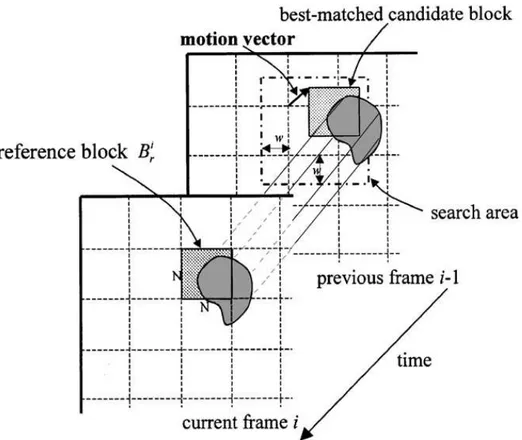
Each macroblock is compared to a macroblock in the reference frame using some error measure, and the best matching macroblock is selected. The search is conducted over a predetermined search area, also known as search window (SW). A vector, denoting the displacement of the macroblock in the reference frame with respect to the macroblock in the current frame, is determined. This vector is known as motion vector (MV).

5 Figure 2.1: Relation between reference frame, current frame and motion vector

When a previous frame is used as a reference, the prediction is referred to as forward prediction. If the reference frame is a future frame, then the prediction is referred to as backwards prediction. Backwards prediction is typically used with forward prediction, and this is referred to as bidirectional prediction.

6

2.3.1. Error Function for Block-Matching Algorithms

Block-matching process is performed on the basis of the minimum distortion. In many algorithms SAD, sum of absolute differences, function is adopted as the block

distortion measure. Assume MBri(m,n)is the reference block of size NxN pixels

whose upper most left pixel is at the location (m,n)of the current frame i , and

) , ( 1 v n u m MBri + +

− _{is a candidate block within the SW of the previous frame}

1

−

i

with ( vu, )displacement from MB . Let ri wbe the maximum motion displacement

and pi(m,n)be pixel value at location(m,n)in frame i , then the SAD between i

r MB and MBri−1 is defined as

∑∑

The SAD is computed for each candidate block within the SW. A block with the

minimum SAD is considered the best-matched block, and the value ( vu, )for the

best-matched block is called motion vector. That is, motion vector (MV) is given by

) , ( min | ) , (u v _SADuv MV = . (2.2)

2.3.2 Full Search (FS) Algorithm

The full search algorithm is the most straightforward brute-force ME algorithm. It matches all possible candidates within the SW. This means that it is at least as accurate (in terms of distortion) as any other block motion estimation algorithm. However, that accuracy comes at the cost of a large number of memory operations and computations. FS is rarely used today, but it remains useful as a benchmark for comparison with other algorithms.

7

2.3.3. Three Step Search (TSS) Algorithm

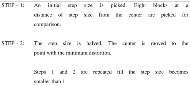
This algorithm is introduced by Koga (1981, p. G.5.3.1 - G.5.3.4). It became very popular because of its simplicity, robust and near optimal performance. It searches for the best motion vectors in a coarse to fine search pattern. The algorithm may be described as:

Table 2.1: TSS algorithm

STEP – 1: An initial step size is picked. Eight blocks at a

distance of step size from the center are picked for comparison.

STEP – 2: The step size is halved. The center is moved to the

point with the minimum distortion.

Steps 1 and 2 are repeated till the step size becomes smaller than 1.

One problem that occurs with the TSS is that it uses a uniformly allocated checking point pattern in the first step, which becomes inefficient for small motion estimation.

2.3.4. Two Dimensional Logarithmic (TDL) Search Algorithm

This algorithm was introduced by Jain and Jain (1981, pp. 1799 – 1808) around the same time that the 3SS was introduced and is closely related to it. Although this algorithm requires more steps than the 3SS, it can be more accurate, especially when the search window is large. The algorithm may be described as:

Table 2.2: TDL algorithm

STEP – 1: Pick an initial step size. Look at the block at the center and the four

8

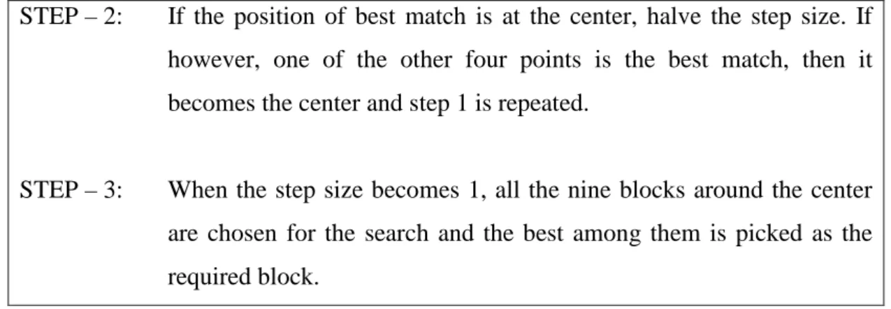
STEP – 2: If the position of best match is at the center, halve the step size. If

however, one of the other four points is the best match, then it becomes the center and step 1 is repeated.

STEP – 3: When the step size becomes 1, all the nine blocks around the center

are chosen for the search and the best among them is picked as the

required block.

A lot of variations of this algorithm exist and they differ mainly in the way in which the step size is changed. Some people argue that the step size should be halved at every stage. On the other hand, some people believe that the step size should also be halved if an edge of the SW is reached. However, this idea has been found to fail sometimes.

2.3.5. Four Step Search (FSS) Algorithm

This block matching algorithm was proposed by Po and Ma (1996, pp. 313-317). It is based on the real world image sequence’s characteristics of center-biased motion. The algorithm is started with a nine point comparison and then the selection of points for comparison is based on the following algorithm:

Table 2.3: FSS algorithm

STEP – 1: Start with a step size of 2. Pick nine points around the SW center.

Calculate the distortion and find the point with the smallest distortion. If this point is found to be the center of the searching area go to step 4, otherwise go to step 2.

STEP – 2: Move the center to the point with the smallest distortion. The step

size is maintained at 2. The search pattern depends on the position of previous minimum distortion.

9

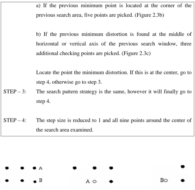
a) If the previous minimum point is located at the corner of the previous search area, five points are picked. (Figure 2.3b)

b) If the previous minimum distortion is found at the middle of horizontal or vertical axis of the previous search window, three additional checking points are picked. (Figure 2.3c)

Locate the point the minimum distortion. If this is at the center, go to step 4, otherwise go to step 3.

STEP – 3: The search pattern strategy is the same, however it will finally go to

step 4.

STEP – 4: The step size is reduced to 1 and all nine points around the center of

the search area examined.

(a) (b) (c)

Figure 2.3: Illustration of selection of blocks for different cases is FSS

(a) Initial Configuration. (b) If point A has minimum distortion, pick given five points. (c) If point B has minimum distortion, pick given three points.

The computational complexity of the FSS is less than that of the TSS, while the performance in terms of quality is better. It is also more robust than the TSS and it maintains its performance for image sequence with complex movements like camera zooming and fast motion. Hence it is a very attractive strategy for motion estimation.

10

2.3.6. Orthogonal Search Algorithm (OSA)

Puri, Hang and Schilling (1987, pp. 1063 – 1066) introduced the algorithm as a hybrid of the TSS and TDL algorithms. Vertical stage is followed by a horizontal stage to search the optimal block. Steps of algorithm may be listed as follows:

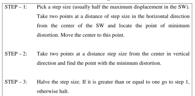
Table 2.4: OSA algorithm

STEP – 1: Pick a step size (usually half the maximum displacement in the SW).

Take two points at a distance of step size in the horizontal direction from the center of the SW and locate the point of minimum distortion. Move the center to this point.

STEP – 2: Take two points at a distance step size from the center in vertical

direction and find the point with the minimum distortion.

STEP – 3: Halve the step size. If it is greater than or equal to one go to step 1,

otherwise halt.

2.4. 3-D RECURSIVE SEARCH BLOCK MATCHING ALGORITHM

Several algorithms, including the algorithms mentioned previous section, have been proposed for frame rate conversion for consumer television applications. There exists a common problem due to complexity of the motion estimator while VLSI implementation of these algorithms; on the other hand, the existing simpler algorithms, such as One-At-a-Time Search (OTS) Algorithm of Srinivasan and Rao (1985, pp. 888 – 896), cause very unnatural artifacts.

De Haan, Biezen, Huijgen and Ojo (1993, pp. 368 – 379) proposed a new recursive block-matching motion estimation algorithm, called 3-D Recursive Search Block-Matching Algorithm. Measured with criteria relevant for the FRC application, this algorithm is shown to have a superior performance over alternative algorithms, with a significantly less complexity.

11

2.4.1. 1-D Recursive Search

The block-matching algorithms, as the most attractive for VLSI implement, limit number of candidate vectors to be evaluated. This can be realized through recursively optimizing a previously found vector, which can be either spatially or temporally neighboring result.

If spatially and temporally neighboring MVs are believed to predict the displacement reliably, a recursive algorithm should enable true ME, if the amount of updates are around the prediction vector is limited to a minimum. The spatial prediction was excluded for the candidate set:

            ± ∨      ± = + = ∈ = − L L U U t X D C CS C t X CSi i 0 0 , ) , ( | ) , ( max 1 (2.3)

where L is the update length, which is measured on the frame grid, X =(X,Y)Tis

the position on the block grid, t is time, and the prediction vector Di−1(X,t)is

selected according to:

{ }

{

}

and the candidate set is limited to a set CSmax:

{

}

CSmax = |− ≤ _x ≤+ ,− ≤ _y ≤+ (2.5)

The resulting estimated MV D( tx, ), which is assigned to all pixel positions,

T

y x

x=( , ) , in the block B( X)of size X×Y with center X :

{

}

)

(X x X X x X X X Y y X Y

12

equals the candidate vector C(X,t)with the smallest error l(C,X,t)_:

{

}

Errors are calculated as summed absolute differences (SAD):

∑

where F( tx, )is the luminance function and T the field period. The block size is

fixed toX =Y =8, although experiments indicate little sensitivity of the algorithm to

this parameter.

2.4.2. 2-D Recursive Search

It is well known that, the convergence can be improved with predictions calculated from a 2-D area or even a 3-D space. In this section, 2-D prediction strategy is introduced that does not dramatically increase the complexity of the hardware.

The essential difficulty with 1-D recursive algorithm is that it cannot manage the discontinuities at the edges of moving objects. The first impression may be that smoothness constraints exclude good step response in a motion estimator. The dilemma of combining smooth vector fields can be assailed with a good step response.

When the assumption, that the discontinuities in the velocity plane are spaced at a distance that enables convergence of the recursive block matcher in between two discontinuities, the recursive block matcher yields the correct vector value at the first side of the object boundary and begins converging at the opposite side.

13 Figure 2.4: The bidirectional convergence (2-D C) principle

It seems attractive to apply two estimator processes at the same time with the opposite convergence directions (Fig. 2.4). SAD of both vectors can be used for selection. 2-D C is formalized as a process that generates a MV:

   > ≤ = ∈ ∀ )) , , ( ) , , ( ( ), , ( )) , , ( ) , , ( ( ), , ( ) ( : ) ( t X D t X D t X D t X D t X D t X D x D X B x b a b b a a l l l l (2.9) where

∑

∑

while Daand Dbare found in a spatial recursive process prediction vectors

) , (X t Sa : ) , ( ) , (X t D X SD t Sa = a − a (2.12) and S_b(X,t):

14 ) , ( ) , (X t D X SD t S_b = _b − _b (2.13) where b a SD SD ≠ . (2.14)

The two estimators have unequal spatial recursion vectorsSD. One of these

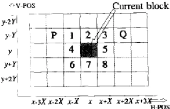
estimators have converged already at the position where the other is yet to do so, that is how 2-D C solves the run-in problem at edges of moving objects, if the two convergence directions are opposite. The attractiveness of a convergence direction varies significantly for hardware (Fig. 2.5). The predictions taken from blocks 1, 2, or 3, are favorable for hardware. Block 4 is less attractive, as it perplexes pipelining of algorithm that the previous result has to be ready before the next can be calculated. Block 5 is not attractive because of reversing the line scan. Blocks 6, 7, and 8 are totally unattractive because of reversing vertical scan direction. Reversing horizontal and vertical scans require extra memories in the hardware.

Figure 2.5: Locations around the current block, from which the estimation result could be used as a spatial prediction vector.

When applying only the preferred blocks, the best implementation of 2-D C results with predictions from blocks 1 and 3. By taking predictions from blocks P and Q, it is possible to enlarged the angle between the convergence direction, however, it is observed worse results rather than blocks 1 and 3 for 2-D C.

15 Figure 2.6: Location of the spatial predictions of estimators a and b with respect

to the current block.

2.4.3. 3-D Recursive Search

Both estimators, a and b, in algorithm produce four candidate vectors each by

updating their spatial predictions Sa(X,t) andSb(X,t). The spatial predictions were

chosen to create two perpendicular diagonal convergence axes:

              − = t Y X X D t X Sa( , ) a , (2.15) and              − − = t Y X X D t X Sb( , ) b , . (2.16)

Due to movements in picture, displacements between two consecutive velocity planes are small compared to MB size. The definition of a third and a forth estimators, c and d, is enabled by this assumption.

Selection of predictions for estimators, c and d, from position 6 and 8 (Fig. 2.5), respectively, creates additional convergence directions opposite to predictions of a and b; however, the resulting design reduces the convergence speed due to temporal component in prediction delays of c and d.

16

Instead of choosing additional estimators, c and d, it is suggested to apply vectors from positions opposite to the spatial prediction position as additional candidates in the already defined estimators to save hardware with the calculation of fewer errors. De Haan (1992) keynotes that; working with fewer candidates reduces the risk of inconsistency.

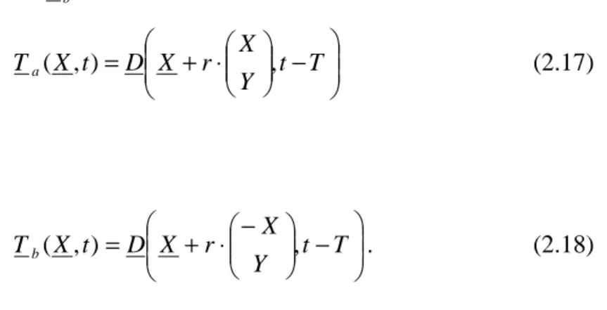
As the algorithm is improved, a fifth candidate in each spatial estimator, a temporal prediction value from previous field accelerates the convergence. These convergence accelerators are taken from a MB shifted diagonally over r MBs and opposite to the

MBs from which S and a S result: b

        −       ⋅ + = t T Y X r X D t X Ta( , ) , (2.17) and         −      − ⋅ + = t T Y X r X D t X Tb( , ) , . (2.18)

By the experimental results, r =2is the best spatial distance for a MB size of 8x8

pixels.

Figure 2.7: The relative positions of the spatial predictors Sa and Sb and the convergence

17

For the resulting algorithm, D_a(X,t) and D_b(X,t)result from estimators, a and b,

calculated in parallel with the candidate setCS : _a

                −       ⋅ + ∪          ± ∨      ± = +                   − = ∈ = T t Y X X D L L U U t Y X X D C CS C t X CSa a , 2 0 0 , , ) , ( max (2.19) and CS : _b                 −      ₋ ⋅ + ∪          ± ∨      _± = +                  ₋ − = ∈ = T t Y X X D L L U U t Y X X D C CS C t X CSb b , 2 0 0 , , ) , ( max (2.20)

while distortions are assigned to candidate vectors using the SAD function (Eq. 2.8).

2.5. GLOBAL MOTION ESTIMATION TECHNIQUE

Camera effects, i.e., panning, tilting, travelling, and zooming, have very regular character causing very smooth MVs compared to the object motion. Zooming with the camera yields MVs, which linearly change with the spatial position. On the other hand, other camera effects generate a uniform MV, called global motion vector, field for the entire video.

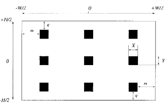
To estimateMVglobal, a sample set S(t), proposed by De Haan and Biezen (1998, pp.

85 – 92), containing nine MVs, D(X,t−1) from different positions X on the MB

grid in a centered window of size (W −2m)Xby (H −2q)Yin the picture with the

width W⋅Xand the height H⋅Yfrom the temporal vector prediction memory

18          − +       − − =          − +       − − = − = Y q H Y q H X X m W X m W X t X D t S y X 2 1 , 0 , 2 1 , 2 1 , 0 , 2 1 ) 1 , ( ) ( (2.21)

where the values of mand q are noncritical.

Figure 2.8: Position of the sample SWs to find MV_global in the image plane

Global motion estimation to find MV_global differs from local motion estimation due to

MB sizes. The MB size related to global motion estimation is fixed toX =Y =16.

Another difference between global and local motion estimations is the algorithm to

find MVs. MV_global is calculated in each SWs by Full Search (FS) Algorithm, on the

other hand, local displacement vectors are calculated by 3-D RS. Although it is possible to choose anyone other block matching algorithms instead of FS to reduce the number of computations, with the very limited number of search windows and

the aim to find more accurate global displacement vector, FS is performed and S(t)

19

The resultant MV_global is derived AS the median vector of each MVs in S(t):

( ) ( )

( )

(

)

(

( ) ( )

( )

)

(

)

global median S S S medianS S S

MV = (2.22)

and added as an additional candidate vector to candidate set in order to use in local motion estimation.

20

3. MOTION ESTIMATION HARDWARE

3.1. VIDEO FORMAT

Wide Extended Graphics Array (WXGA) is one of the non-standard resolutions, derived from the XGA, referring to a resolution of 1366x768. WXGA became the most popular one for the LCD and HD televisions in 2006 for wide screen presentation at an aspect ratio of 16:9. Video frames, whose rate to be converted by the motion estimation and compensation in this master thesis work, have WXGA resolution.

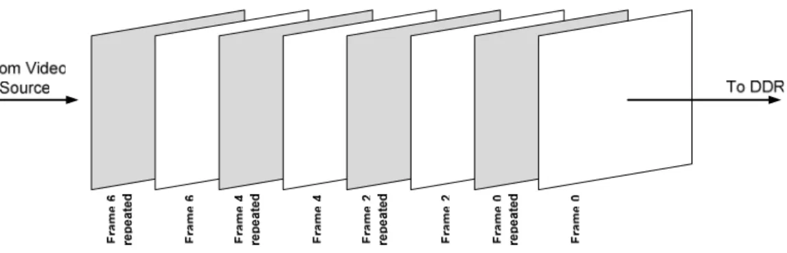
A significant point related to the input video format is that it is composed of consecutive repeated frame of each frame (Fig. 3.1).

Figure 3.1: Video sequence composed of repeated frames

Because each frame is followed by its duplicated copy, it is not necessary to store all the frames provided by video source into memory. Repeated frames are skipped for memory storage, however, they are not completely omitted. Repeated frames are used while outputting the video frames to the display screen.

Table 3.1: Input frame sequence and storage into DDR

Frame Time 0 1 2 3 4 5 6 7 8 9 …

in

F F 0 F 0 F2 F2 F4 F4 F 6 F 6 F 8 F 8 …

in

21

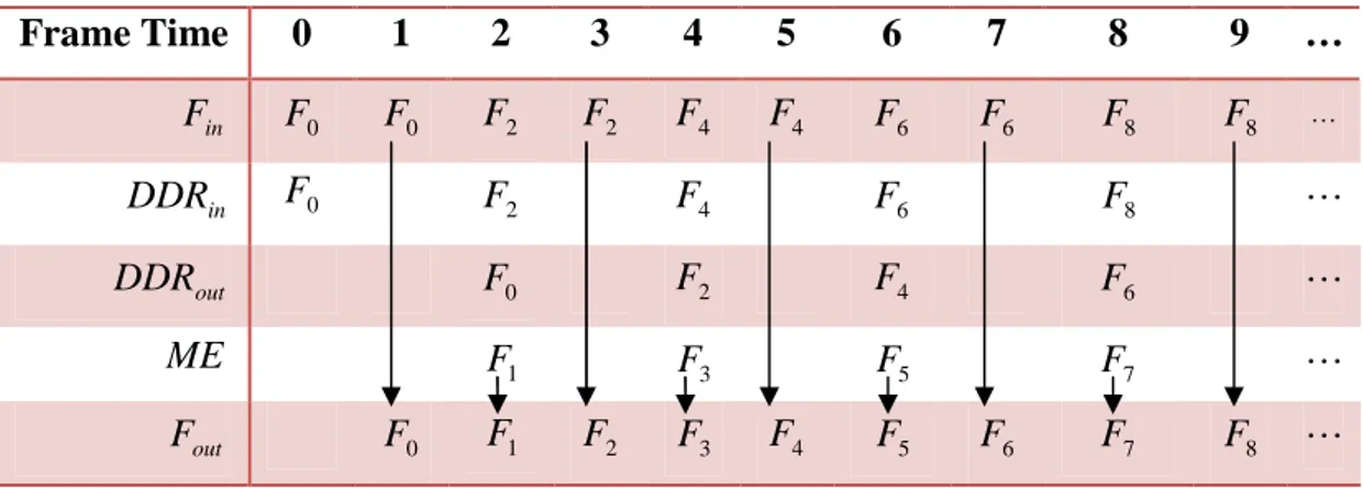
The objective with ME and MC is to generate new sub-frames by interpolation of MBs with MVs instead of repeated frames and outputting the video frames that have a higher frame rate.

Table 3.2: Timeline representation of DDR access, ME, and generation of output video sequence

Frame Time 0 1 2 3 4 5 6 7 8 9 … in F F 0 F 0 F2 F2 F4 F4 F 6 F 6 F 8 F 8 … in DDR F0 F2 F4 F 6 F 8 … out DDR F0 F2 F4 F 6 … ME F₁ F₃ F5 F7 … out F F 0 F1 F2 F3 F4 F5 F 6 F7 F … 8

3.2. HIGH-LEVEL ARCHITECTURE OF HARDWARE

Fully implemented motion estimation and compensation hardware consists of five main components: data converters, external memory block, memory interface, motion estimator, and motion compensator.

Color values of each pixel of a video frame are stored in RGB format in video sources, and digital displayers need also RGB pixel values to show the frames, however, motion estimation algorithms are performed on gray-scaled images. A method to obtain gray-scaled image is to convert the color space into YUV color space, which separates the gray-scale (Y - luminance) and color information (U and V) with the equations

(

)

(

)

(

)

(

)

(

)

(

)

22

To regenerate RGB data from YUV color space for displaying the frame on display screen a reverse conversion is provided using the equations

(

)

(

)

(

)

(

)

(

)

(

)

(

)

(

)

(

)

(

)

(

)

(

)

(

)

An RGB2YUV converter hardware block is placed behind the video source; likewise, a YUV2RGB converter is installed in front of the display screen to convert the pixel values to RGB formats.

RGB2YUV RGBin F ro m V id e o S o u rce DDR i/f YUVin DDR Data Address MOTION ESTIMATOR

GME MEDIAN LME

Ycurrent Yprevious M Vg lo b a l Ycurrent Yprevious MVprevious MVcurrent FRC FRAME GENERATOR YUV2RGB YU Vp re vi o u s Y U Vcu rr e n t YUVout RGBout T o D isp la y S cr e e n MOTION COMPENSATOR

Figure 3.2: High-level block diagram motion estimator/compensator architecture

DDR, as external memory, is used in architecture to store incoming frames and the estimated motion vectors to be used in the following steps of motion estimation.

23

DDR interface block acts as a global bridge in the system and controls the DDR, Motion Estimator and Motion Compensator blocks. DDR interface is the block where the packing strategy of pixels, presented in following section, is operated.

Motion Estimator is the main hardware component of the whole system whose functionality is presented in details following sections.

Motion Compensator is end-point of the architecture where the estimated vectors to be used for interpolation and generation of interframes to increase the frame rate of the original video sequence.

3.3. PACKING STRATEGY OF PIXELS

In architectures for the block-matching algorithms, memory configuration plays an important role. It enables the exploitation of various techniques such as parallelism and pipelining. The motion-estimation techniques are performed with a great amount data during the computations. This requires a decrement in the number of external memory access and fetching more pixels from DDR at a single cycle.

Pixels from video source are received one by one every pixel clock and converted into YUV color space. Instead of storing 24-bit YUV value of each pixel into each word of external memory, every YUV value is divided into 8-bit Y, which is the only value of pixel used in motion estimation, and 16-bit UV block and for four consecutive pixels 8-bit Y values and 16-bit UV values are buffered in DDR interface. Four pieces of Y values are combined to get a 32-bit word; likewise, two pieces of UV values, selected according to 4:2:2 co-sited sampling, are combined to yield another 32-bit word, and then these words are stored to related address of external memory. This configuration of memory provides the motion estimator to fetch luminance values of four consecutive pixels at a single access to external memory.

24

Ri Gi Bi

Ri+1 Gi+1 Bi+1

Ri+2 Gi+2 Bi+2

Ri+3 Gi+3 Bi+3

Yi Ui Vi

Yi+1 Ui+1 Vi+1

Yi+2 Ui+2 Vi+2

Yi+3 Ui+3 Vi+3

Yi Yi+1 Yi+2 Yi+3

Ui Ui+2

RGB2YUV process

Packing process

Ri+4 Gi+4 Bi+4

Ri+5 Gi+5 Bi+5

Ri+6 Gi+6 Bi+6

Ri+7 Gi+7 Bi+7

Yi+4 Ui+4 Vi+4

Yi+5 Ui+5 Vi+5

Yi+6 Ui+6 Vi+6

Yi+7 Ui+7 Vi+7

Yi+4 Yi+5 Yi+6 Yi+7

Ui+4 Ui+6 Storage process DDR Pixel Time t t+1 t+2 t+3 t+4 t+5 t+6 t+7 Vi+4 Vi+6 Vi Vi+2

Figure 3.3: Packing strategy of pixels and DDR storage

3.4. GLOBAL MOTION ESTIMATOR

Global motion estimator is the component to detect the global movements in the background image of frame as a result of camera effects. It is based on FS block-matching strategy on fixed reference locations of each frame and extracting a global MV after scanning the reference SWs.

25

3.4.1. GME Memory Structure

FS block-matching algorithm is performed between current frame with the MB of 16x16 in size and previous frame with the SW of 48x36 in size, calculated with the search range of ±16 in horizontal and ±10 in vertical.

To reduce the number of access to external memory, MB and SW are totally fetched to internal memories, i.e. Block RAMs of FPGA, before the FS is started. The structure of the DDR words, internal block-RAMs is set to 32-bit in width. Because each word consists of four luminance values, the numbers of addresses of SW block

RAM and MB block RAM are set to

(

)

4 36 48 = × and

(

)

(Current Macro Block – Controller – Address Generator)

CURR_MB_BRAM

(Current Macro Block Block RAM -# of Adresses: 64 RAM Width: 32 bits)

SW_CAG

(Search Window – Controller – Address Generator)

SW_BRAM

(Search Window Block RAM -# of Adresses: 512 RAM Width: 32 bits)

SW_DUP_CAG

(Search Window Duplicated – Controller – Address Generator)

SW_DUP_BRAM

(Search Window Duplicated Block RAM -# of Adresses: 512 RAM Width: 32 bits) curr_mg_cag_status pxl_clk sw_cag_status curr_mb_write_enable curr_mb_write_address curr_mb_read_address sw_write_enable sw_enable_a sw_enable_b sw_address_a sw_address_b Y_previous Y_current pxl_clk pxl_clk pxl_clk pxl_clk pxl_clk sw_dup_write_enable sw_dup_write_address sw_dup_read_address READ_BYTE_ SELECTOR curr_mb_data sw_data_a sw_data_b sw_dup_data C_i S_0 S_1 S_2 pxl_clk

26

Three luminance values of SW are required to provide the regularity of the data flow to processing elements in FS algorithm; however, a single block-RAM is eligible to provide two pixel data, S_0 and S_1, over its one read and one read/write ports. So an additional block-RAM, labeled as SW_DUP_BRAM in Fig. 3.5, is installed on global motion estimation structure to transmit the third necessary data, S_2, to processing elements. The contents of additional memory block and the original SW memory block are identical.

READ_BYTE_SELECTOR is a multiplexing structure to select the essential bytes for PEs from the 32-bit outputs of block-RAMs, CURR_MB_BRAM, SW_BRAM, and SW_DUP_BRAM. It decides the luminance to be selected by a simple 2-bit counter inside.

Address generators of block-RAMs are controlled by the status inputs (Table 3.3 and Table 3.4), fed from DDR interface.

Table 3.3: Address generator states

State Number Meaning

0 IDLE

1 WRITE TO BLOCK-RAM

2 READ FROM BLOCK-RAM

Table 3.4: Address generation algorithm

Previous State Current State To Do

0 0 Do nothing

0 1 Enable writing over block-RAM. Reset write

address.

0 2 Enable reading from block-RAM. Reset read

address.

1 0 Disable writing.

1 1 Increase write address by appropriate value.

1 2 Disable writing. Enable reading from

block-RAM. Reset read address.

2 0 Disable reading.

2 1 Unreachable state transition.

2 2 Increase/Decrease read address by appropriate

27 Figure 3.6: GME_MEMO data access timeline and address generation

28

3.4.2. GME Processing Element Array

Due to the search range of ± 16 locations in horizontal, there exists 33 search points for each line of SW. This enables a set of parallel 33 PEs in processing element array structure of global motion estimator. Each PE is assigned to calculate the SAD of the corresponding search location. After a completed calculation PE is assigned for a new SAD calculation of the search location in next line with the same column.

Figure 3.7: Structure of GME processing element

PE array data of SW is provided by the GME memory structure over 3 luminance ports S_0, S_1 and S_2, however, each PE uses only 1 or 2 of this luminance values due to the region of the corresponding its search location. A SW consists of 3 search regions. Columns 0-15, 17-32, 33-48 are defined as region-0, region-1, and region-2, respectively. The data providing of these regions are shared to the luminance ports S_0, S_1, and S_2; on the other hand, the luminance values of current MB are provided over single port, labeled as C_i, in serial and shifted from a PE to the following PE.

29 Table 3.5: Data flow to processing elements over input luminance ports

C_i S_0 S_1 S_2 PE0 PE1 PE2 PE3 PE4 … PE14 PE15 PE16 PE17 PE18 … PE31 PE32

c0 S0,0 x x C0 - S0,0 IDLE IDLE IDLE IDLE … IDLE IDLE IDLE IDLE IDLE … IDLE IDLE

c1 S0,1 x x C1 - S0,1 C0 - S0,1 IDLE IDLE IDLE … IDLE IDLE IDLE IDLE IDLE … IDLE IDLE

c2 S0,2 x x C2 - S0,2 C1 - S0,2 C0 - S0,2 IDLE IDLE … IDLE IDLE IDLE IDLE IDLE … IDLE IDLE

c3 S0,3 x x C3 - S0,3 C2 - S0,3 C1 - S0,3 C0 - S0,3 IDLE … IDLE IDLE IDLE IDLE IDLE … IDLE IDLE

c4 S0,4 x x C4 - S0,4 C3 - S0,4 C2 - S0,4 C1 - S0,4 C0 - S0,4 … IDLE IDLE IDLE IDLE IDLE … IDLE IDLE

c5 S0,5 x x … … … IDLE IDLE IDLE IDLE IDLE … IDLE IDLE

c6 S0,6 x x … IDLE IDLE IDLE IDLE IDLE … IDLE IDLE

c7 S0,7 x x … IDLE IDLE IDLE IDLE IDLE … IDLE IDLE

c8 S0,8 x x … IDLE IDLE IDLE IDLE IDLE … IDLE IDLE

c9 S0,9 x x … IDLE IDLE IDLE IDLE IDLE … IDLE IDLE

c10 S0,10 x x … IDLE IDLE IDLE IDLE IDLE … IDLE IDLE

c11 S0,11 x x … IDLE IDLE IDLE IDLE IDLE … IDLE IDLE

c12 S0,12 x x … IDLE IDLE IDLE IDLE IDLE … IDLE IDLE

c13 S0,13 x x … IDLE IDLE IDLE IDLE IDLE … IDLE IDLE

c14 S0,14 x x … … … … C0 - S0,14 IDLE IDLE IDLE IDLE … IDLE IDLE

c15 S0,15 x x C15 - S0,15 C14 - S0,15 C13 - S0,15C12 - S0,15 C11 - S0,15 … C1 - S0,15 C0 - S0,15 IDLE IDLE IDLE … IDLE IDLE

c16 S1,0 S0,16 x C16 - S1,0 C15 - S0,16 C14 - S0,16C13 - S0,16 C12 - S0,16 … C2 - S0,16 C1 - S0,16 C0 - S0,16 IDLE IDLE … IDLE IDLE

c17 S1,1 S0,17 x C17 - S1,1 C16 - S1,1C15 - S0,17 C14 - S0,17 C13 - S0,17 … C3 - S0,17 C2 - S0,17 C1 - S0,17 C0 - S0,17 IDLE … IDLE IDLE

c18 S1,2 S0,18 x C18 - S1,2 C17 - S1,2 C16 - S1,2 C15 - S0,18 C14 - S0,18 … … IDLE IDLE c19 S1,3 S0,19 x C16 - S1,3 C15 - S0,19 … … IDLE IDLE c20 S1,4 S0,20 x C16 - S1,4 … … IDLE IDLE c21 S1,5 S0,21 x … … IDLE IDLE c22 S1,6 S0,22 x … … IDLE IDLE c23 S1,7 S0,23 x … … IDLE IDLE c24 S1,8 S0,24 x … … IDLE IDLE c25 S1,9 S0,25 x … … IDLE IDLE c26 S1,10 S0,26 x … … IDLE IDLE c27 S1,11 S0,27 x … … IDLE IDLE c28 S1,12 S0,28 x … … IDLE IDLE c29 S1,13 S0,29 x … … IDLE IDLE c30 S1,14 S0,30 x … … IDLE IDLE c31 S1,15 S0,31 x C31 - S1,15 C30 - S1,15 C29 - S1,15 C28 - S1,15 C27 - S1,15 … … C0 - S0,31 IDLE c32 S2,0 S1,16 S0,32 C32 - S2,0 C31 - S1,16 C30 - S1,16 C29 - S1,16 C28 - S1,16 … … C0-S0,32 c33 S2,1 S1,17 S0,33 C32 - S2,1 C31 - S1,17 C30 - S1,17 C29 - S1,17 … … c34 S2,2 S1,18 S0,34 C32 - S2,2 C31 - S1,18 C30 - S1,18 … … c35 S2,3 S1,19 S0,35 C32 - S2,3 C31 - S1,19 … … c36 S2,4 S1,20 S0,36 C32 - S2,4 … … c37 S2,5 S1,21 S0,37 … … c38 S2,6 S1,22 S0,38 … … c39 S2,7 S1,23 S0,39 … … c40 S2,8 S1,24 S0,40 … … c41 S2,9 S1,25 S0,41 … … c42 S2,10 S1,26 S0,42 … … c43 S2,11 S1,27 S0,43 … … c44 S2,12 S1,28 S0,44 … … c45 S2,13 S1,29 S0,45 … … c46 S2,14 S1,30 S0,46 … … c47 S2,15 S1,31 S0,47 … …

INPUT PORTS PROCESSING ELEMENTS

. . . . . . . . . . . . . . . . . . . . . . . . . . . . . . . . . . . . . . . . . . . . . . . . . . . . . . . . . . . . . . . . . . . . . . . . . . . . . . . . . . . . . . . . . . . . . . . . . . . . . . . . . . . . . . . . . . . . . . . . . . . . . . . . . . . . . . . . . . . . . . . . . . . . . . . . . . . . . . . . . .

As it is given in Table 3.5, all processing elements do not use every input port, and ports corresponded to PEs are changing cycle by cycle. This requires an adaptive multiplexing structure for switching between input ports. This structure is built by

30

simple 2×1 multiplexers in front of processing elements and the select inputs of these multiplexers are fed by S_Select port from the GME controller.

Table 3.6: PEs vs. corresponding luminance ports

PE index Corresponding Luminance Ports

0 S_0

1-15 S_0 and S_1

16 S_1

17-31 S_1 and S_2

32 S_2

Figure 3.8: GME PE array structure

Since the MB size is fixed to 16×16, an SAD calculation time equals to 256 cycles for a single search location. Total execution time of PE array for whole SW can be calculated by the formula:

5408 32 21 256 256 _ = ×n+t = × + = TPE array (3.3)

where n is the number of vertical search locations in a SW column, and t is the

31

3.4.3. GME Minimum SAD Comparator

A motion vector in a SW is decided by the location of minimum distortion (SAD). PE array calculates all the SAD values and passes to the minimum SAD comparator component of the GME structure. This component finds the minimum distortion with comparison between incoming SAD value and the SAD value stored in currentMin register. If the comparison results as true, the motion vector is updated by the values of counters, triggered by enable port.

Figure 3.9: Structure of GME minimum SAD comparator

3.5. MEDIAN VECTOR GENERATION

Nine different reference points are set to find the global motion vector defining the

camera movements. Each reference point generates its own motion vector. MVglobal

32

There exists several algorithms to find the median vector; however, due to the clock frequency of input video and the size of chip, it is not feasible to implement a hardware block to find the median vector in a single cycle. In this study, median vector generator is implemented by a serial bubble sorter, which takes:

(

) (

)

cycles in O

( )

Middle element of both x and y components array generates the median vector, said

to be MVglobal.

3.6. LOCAL MOTION ESTIMATOR

By the local motion estimator, it is targeted to find the motion vectors for moving objects. The hardware architecture is based on 3-D RS block-matching algorithm which is explained in Sec. 2.4.

33

3.6.1. Motion Vector Array

3-D RS algorithm is based on the motion vectors calculated during the motion estimation between previous 2 frames.

MV_ARRAY

Figure 3.11: Structure of motion vector array

Local motion vectors are computed by 8 different motion vectors, four of those are directly related to the motion vectors from previous estimation (S_a, S_b, T_a, and T_b). These four vectors are fetched from DDR and stored into the register block of the MV array structure. Two vectors are generated by the updaters. Remaining two vectors are the stationary vector, showing the same search location of MB on SW,

34 Figure 3.12: Structure of updater

Updater blocks inside the MV array generate two new motion vectors to be searched by adding update vectors from an update set:

         −      −                   −      −                      −      −                   −      −             = 4 0 , 0 4 , 4 0 , 0 4 , 3 0 , 0 3 , 3 0 , 0 3 , 2 0 , 0 2 , 2 0 , 0 2 , 1 0 , 0 1 , 1 0 , 0 1 U (3.5)

over spatial vectors, S_a and S_b. The update vectors are listed in a LUT which is fed by a randomly generated update index. The randomization of this index is provided by a pseudo-random number generator, which is designed on the basics of Galois LFSR in this thesis study.

35

3.6.2. LME Memory Structure

Like FS algorithm in GME, 3-D RS is performed between MBs from current frame and the SWs from previous frame; however, the sizes of these blocks differ from GME. MB is set to be 8×8 in size that reduces the size of SW to 40×28 due to the search range of ±16 in horizontal and ±10 in vertical. MB and SW are fetched to internal memories as same as the GME to reduce the number of access to external memory. The configuration of words to write into block-RAMs is also identical to configuration in GME. The only difference related to the block-RAMs is in numbers

of addresses of SW block-RAM and MB block-RAM that are

(

)

4 28 40× ₌ and

( )

, respectively, due to the block sizes.

36

Another difference between the GME and LME memory structures is the width of the output ports. In GME, there exist four output ports, C_i, S_0, S_1, and S_2, of 8 bits in width to run the FS data flow. This enables the calculation of SAD for 33 different search locations. In LME, the strategy of minimum distortion calculation is completely different, where eight blocks in SW, pointed with eight independent motion vectors, are correlated with MB of current frame. This means that the pixels search blocks are not listed consecutively in SW block-RAMs. The situation of the block-RAM configuration prevents the calculation of eight different distortions in parallel with a small number of block-RAMs in structure. Because the number of block-RAMs in FPGAs is very limited, it is necessary to design a structure reducing the block-RAM demand for data providing to processing elements.

To reduce the number of block-RAMs, the parallelism strategy is converted from Parallel-Serial (minimum distortion calculation of different search locations in parallel by feeding PEs with corresponding search pixels of different search locations in serial) to Serial-Parallel (minimum distortion calculation of different search location in serial by feeding PEs with corresponding search pixels of same search location in parallel). The structure can be implemented by two output ports, C and S, each of which is 64 bits in width.

Due to the value of motion vector, that decides the macroblock from SW to be correlated with current MB, eight luminance values of previous MB might be distributed to 2 or 3 words in block-RAM related to search window; on the other hand, the luminance values of current MB are placed in every two words of its own block-RAM. A block-RAM is able to output two values with its one read and one read/write port. This enables that the current MB values can be provided by a single block-RAM; otherwise, for search window, a second block-RAM, with an identical content with original SW block-RAM, is required to provide the data because of the possibility of distribution of necessary values in 3 words due to the MVs.

After fetching these three words from block-RAMs, a multiplexing structure has to be installed behind the block-RAMs to select the correct eight luminance values out of twelve values, fetched from two block-RAMs, due to the MV.