; ' ■ Γ · S '*¿ 5 9 Γ · ν ·'·? г ;·'" -'· ^ -Г ■‘ · τ'* ’* '·’■ ! >·- · Γ - »
LEARNING, INFLATION, AND THE PHILLIPS CURVE
The Institute o f Economics and Social Sciences o f
Bilkent University
by
DUYGU KAPLAN
In Partial Fulfilment o f the Requirements for the Degree o f MASTER OF ECONOMICS in THE DEPARTMENT OF ECONOMICS BiLKliNTUNIVERSrrY ANKARA August 2000
I certify that 1 have read this thesis and have found that it is fully adequate, in scope and in quality, as a thesis for the degree o f Master o f Economics.
<-1
Assistant Professor Dr. Erdem Başçı Supervisor
I certify that I have read this thesis and have found that it is fully adequate, in scope and in quality, as a thesis for the degree o f Master o f Economics.
Assistant Professor Dr. Nedim Alemdar Examining Committee Member
I certify that I have read this thesis and have found that it is fully adequate, in scope and in quality, as a thesis for the degree o f Master o f Economics.
Assistant Professor Dr. Neil Amwine Examining Committee Member
Approval o f the Institute o f Economics and Social Sciences
Prof Dr. Ali Karaosmanoglu Director
ABSTRACT
LEARNING, INFLATION, AND THE PHILLIPS CURVE
Kaplan, Duygu
M.A, Department o f Economics
Supei-visor: Assistant Professor Dr. Erdem Başçı
August 2000
The Replicator Dynamics o f Evolutionary Game Theory is introduced in a closed economy so as to model how a continuum o f firms evolve over time with respect to the pricing strategies. Incorporation- o f Replicator Dynamics facilitates modelling microeconomic frictions that lead to a Phillips Curve on the macroeconomic level. I'he firms are boundedly rational players which are learning, and are apt to make mistakes. Mistakes function as a mutation process and prevent a strategy from becoming extinct. An arbitrary non-empty set o f consumers face a cash-in-advance constraint and total consumption spending is symmetrically affected by changes in growth rate o f money supply which is stochastic. Using a discrete price set, we introduce heterogeneity o f firm behaviour in a single homogenous good market. The economy is simulated ibr a large number o f finitely many time periods. A Phillips Curve type linkage between infiation and output is recognized at stationary states. The slope o f the Phillips Curve is observed to increase as mean o f money growth rate gets higher or as the uncertainty in money growth rate is increased. Slope o f the Phillips Curve diminishes as price stickiness is intensified by either reducing the mistake level or by increasing the firms' responsiveness to relative payoff realizations.
ÖZET
ÖĞRENME, ENFLASYON VE PHILLIPS EĞRİSİ Kaplan, Duygu
Yüksek Lisans, İktisat Bölümü
Tez Yöneticisi; Yardımcı Doçent Dr. Erdem Başçı
Ağustos 2000
Evrimsel Oyun Kuramının öne sürdüğü Replikator Dinamiği kavramı, kapalı bir
ekonomide firmaların fiyatlandırma stratejileri açısından zaman içinde nasıl
evrimleştiğini tanımlamak için kullanılmıştır. Firmalar öğrenen, ancak hata yapan kısmen rasyonel oyunculardır. Hatalar mutasyon sürecini sağlar ve popülasyonda herhangi bir stratejinin yok olmasını önler. Boş olmayan herhangi bir tüketiciler kümesinde, bir ön-ödeme kısıtı çerçevesinde, toplam tüketim harcamaları para arzının büyüme hızındaki stokastik davranıştan simetrik olarak etkilenir. Sürekli olmayan fiyatlandırma stratejileri kümesi, tek ve homojen mal piyasasında farklı firma davranışlarının modellenmesini sağlar. Ekonomi, sonlu ancak büyük sayıda ardışık dönem için simule edilmiştir. Ulaşılan durağan durumda enflasyon ve üretim arasında Phillips Eğrisinin öne sürdüğü pozitif ilişki görülmüştür. Ortalama para büyümesi hızı ya da para büyümesindeki belirsizlik arttıkça eğrinin eğimi artar. Öte yandan, firmaların tcpkisclliği arttırıldığında ya da hata oranlan azaltıldığında Phillips eğrisinin eğiminde azalma gözlemlenmiştir.
ACKNOWLEDGMENTS
I am indebtedly grateful to Assist. Prof Erdem Başçı for his perfect guidance, support, and tolerance throughout the whole course o f this study. I am very privileged to have the chance o f working with such a supportive and encouraging supervisor whose invaluable suggestions and comments made this thesis possible. I also would like to thank Assist. Prof Nedim Alemdar and Assist. Prof Neil Arnwine for showing keen interest to the subject matter and accepting to review this thesis.
I especially would like to thank my friends who have made the last six years o f mine at Bilkent so precious and given me the reason to go on:
Z. Canan Aydemir, for knowing how to listen though I don't know how to speak, for being so close ever,
H. Çağrı Sağlam, for his friendship which has always been so invaluable: sharing, understanding, and inspiring,
F. Senem Erdem, for her joy o f life, and 'delicious' mother-care that she never keeps away,
M. Eray Yücel, for his brotherhood all along the way.
Aytaç, Ali, Serkan, Olcay, and Alper, for their incredible sense o f humour.
Onar, Yeliz, Sündüz, Gonca, and Aytcn, for our late night and early morning talks over coffee and maybe not so coffee.
Ayça, Özlem, Umut, and Nur, for their caring and supportive companion.
Finally, 1 owe much to my parents who keep on saying 'You can', and my one and only brother, smiling, 'But, you ask for it!'.
ABSTRACT ... iii ÖZET ...iv ACKNOWLEDGMENTS ... v TABLE OF CONTENTS ... vi LIST OF TABLES...viii LIST OF FIGURES... ix CHAPTER I: INTRODUCTION ... 1
CHAPTER II: LITERATURE SURVEY ... 5
2.1 On the Theory o f Money-Output Trade-off: New Classical vs New Keynesians... 5
2.1.1 Menu-Cost Models...10
2.1.2 State-Dependent Pricing...12
2.1.3 Limited Participation and Cash-in-Advance Models... 14
2.2 On Evolutionary Approach and Replicator Dynamics... 16
CHAPTER III: THE MODEL ... 20
CHAPTER IV: RESULTS ... 26
4.1 The Stationary State and the Irrelevance o f Initial Distribution... 26
4.2 Effects o f the Mean o f Money Growth Rate...30
4.3 Effects o f the Volatility o f Money Growth Rate... 33
4.4 Effects o f Firms' Mistake Level...35
4.5 Effects o f the Responsiveness Parameter... 38
TABLE OF CONTENTS
CHAPTER V: CONCLUSION ...40 BIBLIOGRAPHY ... 44 APPENDICES
A. TABLES...53 B. FIGURES...58
1. Standard Deviation and Mean o f Density o f Each Strategy at Stationary
State under Different Volatility...54 2. Regressions o f Inflation on Real Output at Stationary State...55
3. Standard Deviation and Mean o f Density o f Each Strategy at Stationary
State under Different Initial Distribution... 56
4. Regression Results for Increasing Mean o f Money Growth Rate... 57
1. Behaviour o f the Economy (|x=0, a=0.0001)...59
1.1. Behaviour o f the Economy (|J.=0, a=0.001)...60
1.2. Behaviour o f the Economy ([.i-O, a=0.005)...61
2. Behaviour o f the Economy (|.i=0,a=0.0001, Initial Distribution Left Skewed...62
3. Behaviour o f the Economy (|.i=0,a=0.0001, Initial Distribution Normal)... 63
4. Inflation versus Real Output During T ... 64
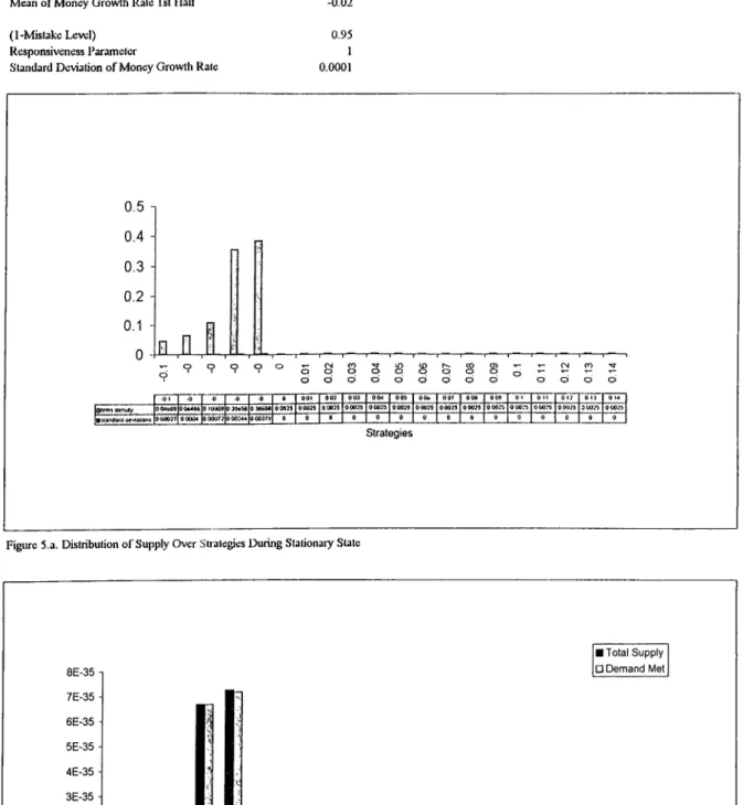
5. Distribution at Stationary State (p=-0.02, o^O.OOOl)...65
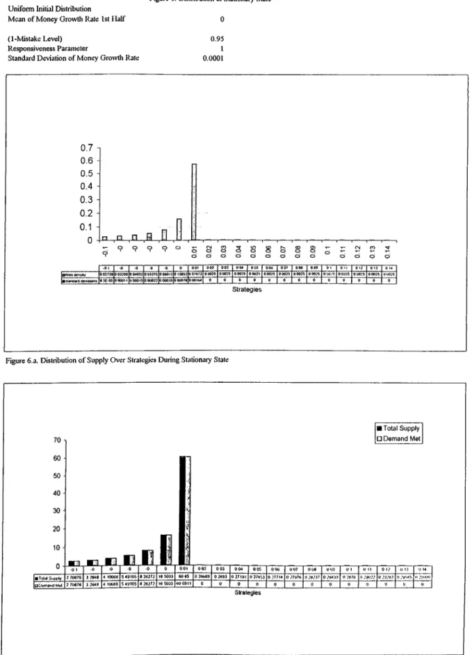
6. Distribution at Stationary State (p=0, a=0.0001)... 66
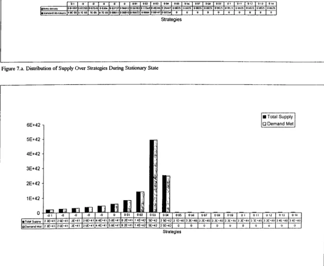
7. Distribution at Stationary State (p=0.02, a=0.0001)...67
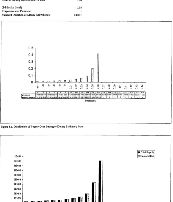
8. Distribution at Stationary State (p,=0.04, a=0.0001)...68
9. Distribution at Stationary State (p=0, o=0.0001, 6=0)...69
10. Distribution at Stationary State (p=0, a=0.0001, 5=0.01)...70
11. Effects o f Increasing the Mean o f Money Growth Rate on the Stationary State... 71
12. Behaviour o f the Economy (p: Stepwise Decreasing, a=0.0001, 6=0.1)... 72
13. Behaviour o f the Economy (p: Stepwise Increasing, a=0.0001,6=0.1)... 73
14. Behaviour o f the Economy (p: Stepwise Increasing, a=0.0001,5 = 0 .2 )... 74
15. Behaviour o f the Economy (p: Stepwise Increasing, o=0.0001,6=0.4)... 75
16. Distribution at Stationary State (p=0, a=0.005, 6=0.05)... 76
17. Distribution at Stationary State (p=0, a=0.001, 6=0.05)... 77
18. Distribution at Stationary State (p=0, o=0.0005, 5=0.05)... 78
19. Effects o f Increasing Volatility on the Stationary State... 79
20. Distribution at Stationary State (p=0, a=0.0001, 6=0.1)... 80
LIST OF FIGURES
21. Distribution at Stationary State (|J.=0, a=0.0001, 6=0.15)... 81
22. Distribution at Stationary State ([.i=0, a=0.0001, 5=0.2)... 82
23. Effects o f Decreasing the Mistake Level on the Stationary State... 83
24. Distribution at Stationary State (|J.=0, a=0.0001, 6=0.05, y= 0.001)... 84
25. Distribution at Stationary State (|.i=0, a=0.0001, 5=0.05, y= 10)... 85
26. Behaviour o f the Economy (|.i=0, 0=0.0001, 6=0.05, y= 10)... 86
27. Behaviour o f the Economy (j.i=0, a=0.0001, 6=0.01, y= 1)... 87
28. Effects o f the Responsiveness Parameter on the Stationary State (5=0.4)... 88
Chapter 1
Introduction
The literature on money-output trade-off and Pliillii)s curv(i is extreiiudy vast. The controversy on the answers to the question ‘Is money neutral?’ leads to a wide literature of both theoretical and ernprical studies with clashing conclu sions. Lucas (1972, 1973) claims only unexpected monetary policy cmn have real effects. On the other hand, ovcrlapi)ing contract models ('I'aylor, 1979), sticky price models (Rotemberg 1982, 1994; Blanchard, 1990), and limitcid participation models (Grossman and Weiss, 1983; Rotemberg, 1984; Alvarc'/, and Atkeson, 1997) generate real effects of money. CocTraiui (1998) i)oints out that, even Lucas’ (1972) model generates effects of anticipatc'd money if money is injectcid by propoitional transfer, d'lui lil,(!iatui(; on nominal G.NP targetting (Feldstein and Stock, 1994: Hall and Mankiw,1994) favour tlu' real effects of monetary disturbances. Still, the cash-in-advanc(' models with
yield more traditional coiiseciueiices of anticipated and nna.nticii)ated inomiy. Römer and Römer (1994) claim that systematic i)olicy endcid ix)st\var re cessions. They also investigatcid the real effects of moiHitaiy disturbance's in post-war US monetary history, identifying six ejoisodes wluu'ei tlu! FcMleral Rxiserve attem])ted to crea,te a recession to reduce! inflation in R.emu'r anel Re)iner
The i)re)l)lem is still alive. R,ee;ently, Shi (1998), Karras anel Ste>kes (1999), Le)o anel Lastrapeis (1998), Keiating anel Nye (1999), Ce)chraii(! (1998), Swan son (1998), nine and Bisedioff (1998) focus on the money-e)utput re!latie)u thre)ngh emprical analysers. Cooley and Quaelrini (1999) prese:nt a Ne'oclassi- cal model e)f the Phillips curve relation.
In this tluisis, we! e:e)nstruct a frame:wenk wliiedi incorporate's the! ie:plicat,e)r dynamiers of the evolutionary ai)proach, in a small e;lose'el ece)nomy subje'e;( to stochastic shoe:ks in nioneiy growth. The agents consist e)f a e:e)ntinuum ed' firms anel an arbitrary non-empty set of consumers. The firms are bemnele!elly rational anel are aj)t to make mistakers in their i)ricing ele!e:isie)iis. Ce)nsume!rs fae:e a cash-in-advance constraint and are fully rational in the! se'nse that theiy spe!nel all the mone!y theiy hold, as long as sni)])ly is available'. Tlie'v start purchasing frenn the h)we!st price. The:refore!, the! shoe ks te> the' me'an of money gre)wth rate are! e)bserveel by the firms as nenninal ele!inanel she)e;ks. There euxists one! he)nioge!iieons gooel, proeliie:e!el anel solel by a he'tere)ge'ne)us set of firms which are differentiated in their pricing de'e;.isie)ns.
Assuming tluvt, a iirm will iiicrcasc its i)iice according (.o Uic inilaUon expec tation it holds, the firms and consumers, repeatedly come togxitlier and j)lay a game. At each period, the distribution of firms over the availal)le i)ricing strategies are updated according to the replicator dynamics of (evolutionary game theory, the formulation of which is due to Taylor and .lonkc'r (1978). The replicator dynamics we use liere, relates the i)ercentage changie in thee density of firms following a certain strategy in a given p(eriod to tine ratio of the payoff from that strategy to the average payoff of the society in that period. The set of possible inflation expectation is exogenous, tlnnefore, the firms’ prices are to be discretely determined in each period.
Introducing the mistake level in the economy, a certain share of the jiopu- lation is distributed uniformly over all the strategies in each [leriod, r(!gardless of previous period’s ¡layoff realizations. Analogous to the mutation ¡nociiss
of the evolutionary approach, the mistakes jirevent any of the varic'ties, \.c.
the strategies in the model, from getting extinct. The firms ¡K'rcc'ive theur own payoff, which is an increasing function of their profit realizations. At any given period, the distribution of the firms over the finite set of strategies describes the state of the world. Given the state of th(( world, the aggr(!gate price level in the economy is a.verag(id oven- the ¡n iccis of tlui goods sold in that period. Besides, the real ¡nofits are calculated by dividing the profits of a tyiie of linn by the previous period’s aggicgatci pricci l(>v(T 'riui ¡noductions costs are assumed to be zero up to a unit ca|)acity.
tion of replicator cl3oiainics from the evolutionary approach. Simulating such an economy, it is aimed to identify whether a stationary state is reaclu'.d or not, at which a positive relation between money and output is observed. Af ter demonstrating the emergence of a Phillips curve type ndationslni) during the stationary state of the economy, the focus will be on the behaviour of the economy undcu· various parameter si)ecifications of the model.
In Chapter 2, a more detailed literature survey is i)res(mt(id. Tlui mode;! is introduced in Chai)ter 3. The results on the behaviour of the economy is described, through succe.ssive simulations under diilVircnt i)araniet(!r specifi cations, in Chapter 4. Chapter 5 concludes.
Chapter 2
Literature Survey
2.1
On the Theory of Money-Output Trade
off: New Classicals vs New Keynesians
The question of whether money is neutral is of central iin})ortance of macroe conomics. The first focus is on whether a change in the level of tlui money stock aflects the real values of any economic varialrles. Tlu! sc'cond is the superneutrality issue concerned with whether a change in tlui rate of growth of the money supply will aflect any real variahhis. N(M)classical ('conomics propose that money is neutral in the long run in the first s('iis(!. Tlu' new classical models of Lucas (1973, 1975), Sargent (1973, 197C), Sargent and Wallace (1975, 1976) and Barro (1976) conclude that anticipated mono'y
nal expectations assumption. On the snpenieutrality analysis, Tobin (19C5) suggested that changes in the inflation rate can affect the time path of the capital stock through influencing the real rate of return on nominal money balances. Keynesian macroeconomics are advocates of the idea that nominal demand shocks produce real effects, implicit is the notion that nominal wagci and price rigidities induce the economy to depart from full-employment'. Defina (1991) i)oints out that rationales for those rigidities have been ad hoc and thus have detracted from the theory’s ap[)eal. Models have been generated in which nominal rigidities appear (hie to agents’ o])timi'/,ing be haviour. Ball, Mankiw and Römer (1988) (henceforth B M ll) suggested an attractive theorjc According to BMR, firms are able to set jirices, but at some costs, and so, price changes are not frequent. Moreover, only a fraction of all firms change prices at a time. The BMR model leads to aggregate ¡nice rigidities, so that nominal shocks have real effects on the economy. Naish (1986) investigates why money is unlikely to be suiierneutral and ¡nits the blame on the imperfectly flexible prices. As initially siielled out liy Fischer (1977) and Phelps and Taylor (1977), sticky prices and wages induce a sta bilization role for monetary policy. Naish (1986) discusses futherniore that sticky prices have additional eflects, causing the firm’s average hived of ont- ¡)ut to depend on the antici[)ated rate of inflation. That the nominal prices are costly to adjust, most convincingly explains the ¡)ric(! stickiiuiss. Barro (1972) |)ioii(Xired this ai)proach,which is d(ivelo})ed by Sluishinski and Weiss (1977,1979), and Mu.ssa (1981), followed by Sluishinski and Weiss (1983), Roternberg (1982a,b), Kuran (1983a,b) and Danziger (1983, 1984). This lit-
'Lucas (1972), though not rcigarded a.s a Keyne.siaii, also cai)turos tlu! same idea hy his
confusion model.
erature assumes firms do not change prices continuous!}^ since tliere are real menu costs emerging as a by-product of price changes.
The positive relation of high money growth with high real activity at business-cycle frequencies, has also been attributed to tlu' sticky prices. Usu ally, the main reasoning behind monetary noimeutrality is said to Ixi the im plicit or explicit contracts. In the past decade, few similarly explicit model economies have been presented assuming a role for nominal contracts from underlying assumptions about the economic environment and explain the im plications of contract arrangements for money and business cycles. Contract theory could not i)rovide a full justification, therefore the reasons behind sticky prices refer to the costs of price adjustment (Rotemlierg 1982, Park ing 1986) or on the multiplicity of rational-expectations eiiuilibria (A'/ariadis and Cooper, 1985b). Setting up a model which is a variant of Lucas (1972), Haubrich and King (1992) assume monetary changes are neutral toward real aggregates in the absence of contracts since economic agents accurately per ceive the changes. A Phillips curve emerges under two conditions: an in teraction of individual and aggregate uncertainty and an incomiileteness of markets, which is due to private information. Their results depend more on the existence of market incomiileteness than on specific rationale. Not all of the literature attempts to explain Phillips curve with sticky prices. In Farmer (1988) credit is taken to play the role for tlu; transmission m(;cha- nism. Much of the literature however tries to justify the sticky prices and wages led by the Gray (1976), Fisher (1977), and Taylor (1980). On the other hand, the bubble (self-fulfilling prophecy) literature attempts to ex
ena as market based occurrences tliat depend on expectations, not contracts (Azariadis and Guesnerie, 1986). Keeping the prices sticky but not fixed, the model of Haubrich and King (1992) generates a Phillips curv(i so that they examine the slope of the Phillips curve when the monetary variability is changed. Their results contradicts Barro’s (1976) statement that (dficient competitive contracts nectissarily reduce the dependence of output on nom inal money growth. Suppliers set prices before demand is realized and high money growth induces high output, a possible reasoning for which may b(i the insufficient adjiistement of prices. Defina (1991) tests the BMP, model empirically by focusing on a key prediction, the degree to which nominal shocks affect output varies inversely with the level of trend, namely, infla tion. As inflation happens to increase, firms’ ¡)iofit niaximising prices change more quickly on average. Since higher inflation causes more frequent price adjustment implying less rigidity, nominal shocks have smaller real (dlects as inflation gets higher.
Howciver, main theories of macroeconomics which ])ropose an output- inflation trade-off do not permit average inflation to have an effect on tlui trade-off including the imperfect inlormation model of Lucas (1973), attribut ing no real effects for nominal rigidities, and the traditional Keynesian mod els. The Keynesian models incorporate nominal rigidities, still, k(H'))ing the extent of rigidity fixed. Thus, the trade-oil is not d(!])end(int on tlu; clianges in the inflation rate. B M R’s negative impact thus i)rovid(is an alt(irnative to the prominent theories.
forty-three industrialized countries questioning tlie BMR thesis, while allowing the suggested pricing behaviour to vary in importance from country to countr}'. He states “If ‘menu costs’ are a strong and pervasive influence on ıtrice flex ibility, evidence that average inflation matters should arise; in a significant fraction of countries.” He concludes that average inflation has a negative and significant effect on the trade-off in a large fraction of countries. The result are aligned with cross-country study of BMR and US time, scries evidence; e)f Evans (1989). Beside;s, Sachs (1980) derives econometric Phillis curve esti mates, and identifies a decrease in the slope of the Phillips curve after the' World war II. He suggests that the public expected the monetary authoritie;s to take action so as to prevent price deflations and unemiiloyment anel the; long-term contracts were common. Therefore, higher rigiditie;s existe;el, which led to a diminishing slope of the Phillips curve.
The; BMR model preepeises that nominal shocks have smalle;r re'al e'ffe'e'.ts as the variance of aggregate shocks becomes higher. With increasing variability, firms’ profit maximising prices become more uncertain. Therefore;, firms tenel to pursue more flexible pricing strategieis. Defina (1991) concludes “since Lucas (1973) model is consistent with the; same inverse relation, the predicteel role of aggregate variability cannot be used to validate the BM R model. But sine;e; average; inflation anel aggregate variability e'e>ulel be e;e)ne'la(e'el, strong e;vielence for the BMR thesis reeiuire;s ave;rage; inflatie)n te> ma.tte;r afte;r accounting for variability.
the implications for the monetary policy. To sum uj)
2.
Their theory implies that the lower average injlation falls, the more, ■responsive 'is output to nominal shocks, s'ach as changes vn money g'lmuth. Hence, initial declmes in mpid 'i'liflatio'ii etiyi- neerred by a central bank might carry 7'elatively small output costs, b'ut attempts to eliminate inflation could beco'ine extremely expen sive.
B M R ’s fundamental results are implied by the central Keynesian theories in which the degree of rigidity is endogenous, including the state-dependent
pricing models In contrast, Caplin and Si)ulber (1987) i)rovide an example
of a menu-cost model with predictions contradicting the BMR.
2.1.1
Menu Cost Models
)r
• h .
New Keynesian models of the business cycle ha.vc tried to mod(d price rigidi ties consistent with fully rational optjmizing behaviour and focus on the effects of ridigitics on the fluctuations of the economy. Iflielps and Tayh (1977) followed by McCallum (1977,1986), opiuKul tlui road for this apinoacl The material costs of price adjustment due to uiia,ntic.ii)at(!(l shocks arc; i(!f- ered to as ‘ menu costs’'* and Akerlof and Yellen (1985a,b), Mankiw (1985) and Blanchard and Kiyotaki (1987) find significant ex])lanatory power of the
■^Defina(1991), pp. 411-412.
^Sheshinski and Weiss (1977)
menu costs in the theory of business cycles. As Mankiw (1985) and Blan chard and Kiyotaki (1987) conclude that the private costs of price rigidities may be small, but the associated social costs may be quite largci in numerical analyses. The analysis of menu costs typically proceed in a monoi)olistic or monopolistically competitive framework. Caplin and Spull)or (1987) show that the price stickiness and the nonneutrality results disapi)ear in tlu; ag gregate if firms follow (s,S) pricing strategies. Caminal (1992) proves the oiAimality of (s,S) pricing strategies under quite general conditions. Lucke (1995) argues that Caplin and Spulber’s result requires tin; slightly rcistric- tive assumption of a rnonotonically increasing money supply, while the New Keynesian theory of menu costs is intended to cover both positive and nega tive demand shocks, possibly in a random sequence. Moreover, adjustments costs in cases of demand shocks also include costs of changes in input and output quantities in addition to the menu costs.
Lucke (1995) considers the partial eciuilibriurn model of Mankiw (1985), and treats the menu costs in the original set-up. The purpose of the study is to show that the spectacular property of large social externalities induced by small private costs vanishes if factor adjustment costs are taken into account. He concludes that it is questionable to state that the small memi costs gener ate large busine.ss cycles. The result ])ertains to any kind of adjusi nn'iit costs against demand shocks, even when the demand does not follow a. monotiUK! l)attern as specified by Caplin and Spulber (1987). Danziger (1999) studies a dynamic economy with menu costs in a general eciuilibrium set-uj). He finds that the correlation between unanticipated movements in tin' pric(' in
Leahy (1991, 1997) where price distribution, and thus the history of monetary shocks, determines the consequences of monetary surprises.
2.1.2
State-Dependent Pricing
yVmong the vast amount of research focusing on tlie effects of microeconomic frictions on the macroeconomic dynamics, a main focus has been on the (s,S) models initially presented by Arrow, Harris and Marshak (1951). State de pendence of individual decisions becomes the distinguishing feature of this line of research. Agents act when a state variable crosses some critical thrcish- old so that the costs and benefits of adjustment are balanced. Blinder (1981), Caplin (1985), Mosser (1991) in the context of inventory dynamics. Caplin and Spulber (1987), Cabellero and Engel (1991,1993) and Caplin and Leahy (1991) in the context of prices; and by Bertola and Caballero (1990), Ca bellero (1993), and Eberly (1994) in the context of consumer dural)les, anal yse the implications of such microeconomic specification on the aggregates of the economy. Caplin and Leahy (1997) state that one of tlui most limiting aspects of these models is that they focus exclusively on the impact that microeconomic inertia has on the aggregate dynamics, ignoring thii feedback from the aggregates onto individual behaviour. Cai)lin and Li'ahy (1997) exainine the feedback effects with a hybrid of fixed and flexibh; pric(! models. They model the aggregate price level to have an independent effect on firms’ profitability. When aggregate demand has an increasing trend for a certain period of time, the price level becomes flexible in the inflationary direction. If aggregate demand is falling, the price level becomes flexible in tin;
defla-tioiiary direction. Each firms pricing decision affects the i)ricing decisions of others if tlie fcedl:)ack effects are considered. The way in which tlie decisions interact is captured by the degree of strategic complementarity in i^rice set ting. They show tliat increases in the degree of strategic comirlemcntarity increasii the range of output fluctuations and decrease the siz(i of firms’ price adjusl.ments. This contradicts Ball and Römer (1990) where all firms change [)rices at the sanu! time. In Caplin and Leahy (1997), the price changes are staggered. They also show that an incr(!ase in the variance of money supply reduces the slojrn of the Phillips curve as in the irnp(iifect information model of Lucas (1973).
Conlon and Liu (1997) present a generalized (s,S) state-dependent pricing model in which menus are changed, not just in response to price misalign ment, but also in response to factors such as changing ])roduct mix. The model generates aggregate price inertia, and so reverses an important ear lier result on neutrality in state-dependent pricing contexts in more gimeral settings than previous modifications. It also provides a compromise between state- and time-dependent rules gives a glimpse at the dynamic implications of menu-cost models, and reproduces two recent results; one on Phillips cnrv(i slopes, and one on asymmetric fluctuations. The model implies that, as the underlying inflation rises, inertia falls and the Phillips curve' Ix'coiik's ste'c'pi'r, confirming an imi)ortant reisult by Ball et al. (1988). Also, tluiy state; that under positive inflation, accelerations in aggregate demand have smallen· ef fects on output than decelerations, supporting results of Tsiddon (1993), anel Hall and Mankiw (1994).
2.1.3
Limited Participation and Cash-in-Advance M od
els
Monetary economics conventionally argues that an expansionary moiuitary I)olicy generates a short-term decrease in nominal interest rates and an in crease in the level of output. Recently, Lucas (1990) and Fuerst (1992) show how this outcome is likely in a monetary model with a cash-in-advance con straint if there is ‘limited participation’ in financial markets in response to shocks, basing their discussion on the ideas of Grossman and Weiss (1983). ‘Limited Particii>ation’ is sometimes named as portfolio rigidity, meaning that firms and financial intermediaries adjust their financial jrositions more frequently than do the households. Therefore, firms and financial intininedi- aries face the undesirable consequences of unanticipated demand shocks first. This implies that expansionary monetary shocks product! a downward ))res- sure on nominal interest rates by raising the amount of loanable funds that banks have available for lending to firms, thereby leading to an increasci in the real economic activity. In the context of the Luca.s-Fu(!rst fram(iwork,by Christiano (1991) and Christiano and Eichenbaum (1992a,b),the licpiidity effect is illustrated in computational general eciuilibrium models. Yet, tlui liquidity effect is not explained solely by the limited i)articipation assuin])- tion. Recent econometric literature, including Bernanke and Blimhu' (1992) and Cristiano and Eichenbaum (1991) provides enqnrica.1 (widence in su[)port of the existence of a liquidity effect. Cooley and Nam (1998) point out that anticipated inffation effects associated with a money siqiply shock have tlie potential to outweigh the liquidity effect in equilibrium. Nason and Cogiey
(1994) present cases of failure to identify a liquidity effect despite the limited participation assumption.
Lucas-Fuerst style limited participation in a cash-in-advance model does not produce significantly different behaviour of the output resi)onses to a money supply shock, than the pure cash-in-advance model with fidl-participation. Christiano (1991) and Christiano and Eichenbaum (1992a) in addition, as sume that capital also adjusts sluggishly, and Christiano and Eichenbaum (1992b) assume that production is inflexible in order to produce a licjuidity effect. The quantitative models above do not produce persistent liciuidity effects. Christiano and Eichenbaum (1992a) add the additional assumption that there are significant adjustment costs in order to get a more persistent
response of output to monetary shocks. A related paper by Euerst (.ex
tends the limited participation assumption by incori)orating a real financial sector to the Christiano and Eichenbaum monetary model. Fisher (1994) also examines the monetary transmission mechanism in a model which incori)o- rates credit market imperfections and limited participation. In the framework of a standard RBC , Cooley and Narn (1998) include a.symmetric informa tion and limited participation in their rnochd. The standard R13C model has not been successful in producing a propagation mechanism for shocks, like; monetary shocks, that are not inherently i)ersistcnt. Cooh'y and Nam (1998) conclude that a j)Ositive money supply shock gemuates a (hicreasc; in nominal interest rates and an increase in output, while the asymni(itri(( information structure does not amplify or propagate the monetary shocks.
2.2
On Evolutionary Approach and Replica
tor Dynamics
In this soction, we will take a diversion to the evolutionary game theory and related learning literature. In the subseciuent chapters, we will use a similar model to generate a Phillips curve. A full introduction and an oven view of the literatiu'(! can be found in Weibull (1997). The evolutionary apinoach assumes a game in question is played repeatedly many times by boundedly ra tional players who are randomly drawn from large populations and who have little or no information about the game. The agents are Iroundedly rational and not perfectly coordinated. The general characteristics of an evolutionary model is governed by the selection and the mutation dynamics. The scdec- tion process favours some of the varieties over the others and the mutation process creates the varieties, which are actually the strategiiis in a ganui. In a market, the basic selection mechanism is the economic survival, and the mutation process is experimentation, innovation and mistakes. Mainly, the evolutionary approach focuses on how the population distribution of decision rules or strategies behaves over time.
Evolutionary exi)lanations have been considered by social scient ists even before Darwin. VVeibull (1997) points out that Malthus, Marshall, Schum peter, Hayek, and Adam Smith have evolutionary perpiudives in some their writings. In the context oi game theory, John Nash introduced the intepre- tation of ‘mass action interpretation’ . Agents gather emprical information on the relative advantages of the various pure strategies at their disposal.
Evolutioriai'
3
' game theory incorporates the concepts of Evolutionary Sta bility and Replicator Dynamics. The concept of an evolutionarily stable strategy is dne to Maynard Smith and Price (1973), and also Maynard Smith (197-1, 1982). Such a strategy becomes robust to evolutionary processes such that a population playing such a strategy becomes uninvadable by any other strategy. Yet, it docis not explain how a population arrives at that strategy. I'he replicator dynamics, naimily the time derivative of the freciuency of a strategy being c(iual to the stratcigy’s relative ex[)ect('.d payolf, d(^scril)(is the selection process, specifiying how population shares associated with differ ent pure strategies evolve over time, the mathematical formulation of which is due to Taylor and .Jonker (1978). The selection dynamics are treated in two categories: payoff-positive selection dynamics where all pure strategies that perform better than the average payoff have positive growth rates and all pure strategies that perform worse obtain negative growth rat('s; weakly payoff- positive selection dynamics where at least some pnrci strategy that performs better than average, granted that such a strategy exists, has a pos itive growth rate. Literature on the evolutionary approach in game theory is vast. Binrnore and Sarnuelson (1994) discuss the evolution of norms, iden tifying the concept with the equilibrium selection problem in game theory and provide an example on the Ultimatum Game. They stress that adopting an evolutionary ajoproach may induce the economists abandon tlui literat.nr(i on refinements of Nash equilibrium. Bicchieri et al. (1997) also consider the dynamical processes responsible for establishment, maintenancci, meta morphosis, and dissolution of norms. Redondo (1995) and Wiebull (1995) provide source books on evolutionary game tlieoiy.Recent studies have shown that replicator dynamics may result from learning models of the two categories: reinforcement learning (Börgers and Sarin, 1997) and learning by imitation (Schlag 1997). Bush and Mosteller (1951,1955) and Estes (1950) investigate reinforcement learning in the con text of psychology, followed by Lieberrnan (1993) and Walker (1995) re cently. Cross (1973, 1979), Roth and Erev (1995), Brirgers and Sarin (1997), Mookherjee and Sopher (1997), Erev and Roth (1998) and Erev and Rapoport (1998) analyze reinforcement learning in repeated decision cnvironnKuits.
Börgers and Sarin (1997) compare Cross’ (1973) version of Bush’s and Mosteller’s (1951) model with the Taylor two-population dynamics, and con clude that over bounded time intervals, the reinforcement learning process is approximated by the replicator dynamics and there exists a close analogy in between the two. Hoirkins (1999), in a large population where agents are repeatedly drawn and randomly matched, states that the aggregation of the reinforcement learning behaviour yields an aggregate dynamic which belongs to the same class of several ibrmulations of evolutionary dynamics. Schlag (1997) in a set-up where individuals in a finite population rc])eatedly choose among actions yielding uncertain payofis, restricts his search to h'arn- ing rules with limited memory that increase exjrected payoffs regardh'ss of the distribution underlying their realizations. Between choice's, individual observes the action and realized payofl of one other individual. It is shown that the rule that outperforms all others is that which imitates the action of an observed individual whose realized outcome is better than herself, with a probability proportional to the difference in these realizations. When each individual uses this best rule, the aggregate population dynamic is
approx-imatecl by the replicator dynamic. Dawid (1999) also concluded that the evolution of the population strategy is described by the replicator dynamics for an imitation type learning rule.
This thesis incorporates the concept of the replicator dynamics to (Udine the rule of how firms evolve over time with resj^ect to tin; pricing strate gies. We consider the firms as boundedly rational players who are a])t t.o make mistakes. Consumers face a cash-in-advance constraint and total con sumption spending is is symmetrically affected by changers in growth rate; of money siprply. Using a discrete price set, we introduce heterogeiuiity of firm behaviour in a single homogenous good market. The contribution of this study is that the microeconomic frictions inherent in the replicator dynamics model induce a Phillips curve relationship on the macroeconomic UiveT
Chapter 3
The Model
Wo consider a society composed of a coiitimmm of firms and an arbitrary nonempty set of consnmers. Supply of money is stochastic. We assume that consumers face a cash-in-advance constraint and we simulate the (economy such that at discrete time intervals, firms’ sui)ply is purchased with all the money that the consumers hold. Firms pursue different strategies in terms of their pricing decisions and consumers spend all the money they hold as lorig as supply is available. The state of the world is given by the distribution of the firms over the iiricing strategies at time t. The pricing stratc'gies
of the firms vary, depending on their inflation expectations. firm’s type'
is determined by its inflation expectation. Therefore, tlu' set of tyiies is identified and kept constant throughout a given period. Poimlation dmisity of each type evolves over time. Firms are boundedly rational and are apt to make mistakes. At each state of the world, when firms are to update their
beliefs about next period’s inflation, a certain proportion of the firms of each type pick a random pricing strategy regardless of their payoffs. Firms evolve according to a r(hnforcement learning rule. They observe; their own payoff as well as the average payoff of the society at each state. Consumers always remain rational in the sense that they spend all their money starting from the least expensive option until either supply or demand is exhausted. The demand of the consumers is characterized by the total moiuiy sup[)ly. VVe let the firms play the game for a large number of finitely many periods. The initial condition for the state of the world is giv(;n.
Introducing the notation will facilitate the illustration of the model in a
detailed and formal manner. The number of types of firms is given by N,
which represents the number of pure strategies of pricing decisions. Tin; firms are indexed by i, and di^t represents the population density of firms with i)ure strategy i in period t. T is the total number of time periods. Monc'y growth rate is normally distributed around the mean /i with the standard deviation o. ¡It denotes the money growth rate in ])eriod t. Therefore the total money supply in period t is given by
Ml — Mi-\ ·
(1
+ /¿i)A firm of type i has the inflation strategy of Given the i)revious period’s
aggregate price leveF, Pi_i, the nominal supply of firms of tyi)e i in peuiod
^ T his p r ic e in d e x c o n s is ts o f a w eig h ted a v e ra g e o f all fir m s ’ p r ic e s , w eig h ts hcniig eiju al t o d e n s ity o f g o o d s s o ld
t, S i t, equals
Si,i =
^/.-1
■(1
+ Tr'-'i) · di^tTaking the total inoiiey supply Mi as the amount of total demand of the
consumers at period t, the real profit‘d of a single type i firm in period t, R i, IS = < (l + TT^)
0
if Ml -
E t i
>
s,t
i f M t - J 2 [r J i{S k ,i) < 0 I ---— —St.t otherwiseDistinguishing between profits vs perceived payoffs, the lattc'r is g i v e n b y
Uг ,t
=
-
1 where7
>0
is a “responsiveness” parameter.The firms observe their own payoffs in addition to the averagxi payoff in
the society, Ut. Actually they observe
N
= E
j=^
the weighted average of increasing functions of real profits wliich (Kiiial zero in case lli^t is zero. With this set of information, the population density of each type of firms are uptaded according to the replicator dynamic
^ R eal p r o fit is m e a su re d in term s o f p r e v io u s p e r io d ’s g o o d s . N o t e tlia t tlie iir o d u c t io ii c o s ts are ta k en as z e r o u p t o a c a p a c it y o f o n e u n its.
The above equation defines how the distribution of tlie iiriris (;volves over time. The parameters \ — 5 and
7
refer to the mistake level and r(!sponsive-ness parameter resixictively. A 5 of less than T imposes the a,ssnmption that
a certain share of population make mistakes which are nniforml}^ distributed over possible strategies. Thus, even when zero payoff is observed for a pricing strategy, some of the firms keep following it in the following period. On the other hand,
7
, which is identical for each type of firms, is a parameter of the learning ability of the firms. Intuitively, higher values of7
mak(;s perccnved payoffss more pronounced and hence leads to a society of quicker learners as a whole. In order to observe how inflation behaves in the duration of simu lation, we find the aggregate price level in period t as the weighted averagi! of the i)rices of the firms who were able to sell any positive amount in that period.N
Pi = Pt-l l
¿=1
Our definition of the weights, given below, makes tin; above (Hiuation a
weighted average of the j)rices of only the selling firms, d'he mod('l imi)li('s that di^u file density of the type i firms, corresponds to the (piantity supi)li(>d
quantity sold by type i firms at P i_ i(l + Tr'y) is given by
^ <kl. i f w ,
<
0
if M i - E r J i K a< 0
(¡. . . Yl-Y'kYVYf··:
"'Oi .S',, — otherwise
In order to determiiHi the weights of the goods sold at /;, we normaliz(i the ;;q j figures to derive the percentage of goods sold l)y type i firms at P/._i(l +
7
r'·,;). The normalized sales are given byL·k=ı
so that the price index consists of a weighted average of all selling firms prices. Then, given the aggregate price level, and the updated distribution of firms over the inflation strategies, the new supplies of (!a,ch type; of firms are determined. What rimiains is the calculation of tlui inflation obscn vc'd in period t,
TTi = Pt - Pt-v
P>l-[
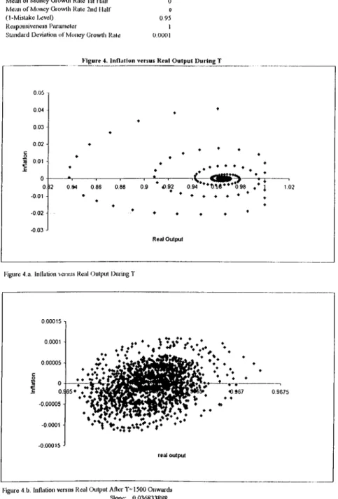
The next liguie that wc will be locusing attention on is tluî nsd out])ut
1(!V(!İ in (!a.ch p(',riod /-, so that w(! will b(i analysing tlui r('lat,ion b('(w('('u in-
llation and real output in our set-up. Real output lev(d, Y, is giv(m by
N
i= l
that the iriaxiiiiuin capacity of real output is constant and equals
1
so t hat the above equation gives a consistent measure of real output. Full employment level therefore corr(;sponds to the case of aggregate real output being equal to 1. Thus, the real output level directly reflects the {'.mployment level in our economy. The ladiaviour of the economy will be observed over time for a duration of T periods. The first question is whether there exists a convergence to stationary state of the economy. If so, the relation between inflation and real output will be (ixamined, (luestioning the presence of a Phillips curv(! tyi)e linkage. The slope of a possible Phillips curve will be investigated. Moreover, the effects of mean and standard deviation of growth rate of money, mistake level, and responsiveness parameter on the stationary state will b(i analyscxl.Chapter 4
Results
4.1
The Stationary State and The Irrelevance
of The Initial Distribution
We simulate the model using Microsoft Excel Workbook facilities. We take T=5000 as for the duration of the simulation. The game is played ixipcatcdly
T times, firms updating their beliefs at each stage and determining their
prices according to the dynamics explicitly described in the i)revious chaptc'r. Our initial concern is whether the model reacluis a stationary state; at souk!
period during the whole duration. We initially divide the whole period into two and observe the standard deviations of the distribution of firms over
the strategies in the second half, T. Throughout the whole analysis, we
strategies, tt'^/ ranging from a deflation rate of -0.05 to an inflation rate of 0.14, incremented by
0
.0 1
. Initial money supply, A/q equals100
while the initial price level, Po is <dso 100.In Table
1
, for money growth rate,/i= 0, mistake level, l-(5= 0.05, responsiveness level, 7= 1, and initial densities, di^i= 0.05 for all i = 1,2,..., N, for different values of standard deviation of money growth, a, the standard
deviations and means of densities are prcisented for T only. Obscn ving the
considerably small figures of standard deviations in T, for different valnes of (j, the standard deviation of the money growth rate, we conclnde that it is appropriate to investigate the relationship between the money growth rate
and real output during T where a stationary behaviour has be(ui ixiacluKl.
For a ranging from 0.0001 to 0.001, we observe that the standard deviations
of the densities remain in the order of maximum
10
~ * for a =0
.0 00 1
.At the bottom of Table
1
, for T, which we identify as Ireing at the sta.tion- ary state, the mean and standard deviation of the inflation and real output figures are also reported. Given the other parameters, w(! observe! variation in the order of10
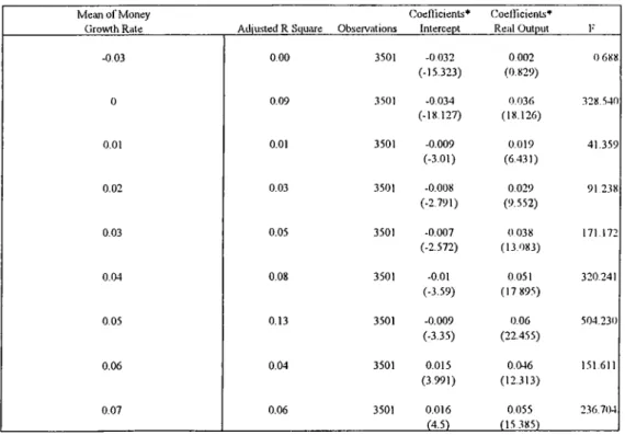
“ '' for the real output figures and the standard d(!via.tion of the inflation at the stationaiy state for <7=0.0001, wluire tlu! mean of infla tion at the stationary state remains unaffected as a is increasc'd. In the last line, the “Slope” item gives the slope of the line wh(!n the inflation is ])lotted against the real output figures during T. The slope of the line is caladatc'd by least squares method for the regressionfor real output at each t in T. Table
2
suininarizes the results of the nigrcs- siori for different ¡i. For negative values of ¡i, the slope happens to be very close to 0, yet statistically insignificant for the case of ¿=0.95. Still, for non- negative values of nician of money growth rate, slope becomes always positive and statistically significant. Besides, the coefficient of real output, namely the slope increases as /i is increased. Table 4 reports regression ixisults for different 5 values. It is observed that as the mistake level is increased in the economy, the slope becomes always positive and statistically significant ev(!ti for negative rates of money growth. Besides, higher slo])e is ol)S(!rved in case of higher mistake level for firms. In Figure1
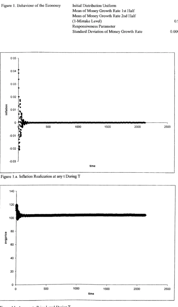
, data is plotted for inflation and the aggregate price level for the whole period. Increasing the volatility in the mean of money growth rate, the behaviour of the economy is illustrated in Figures 1.1 and1
.2
. Volatility of inflation increases and the aggregate price level departs from the initial level of100
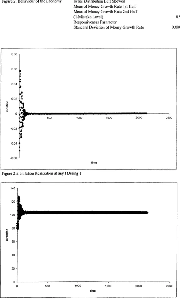
, implying rigidities on tlui aggregate. As Hallman et al. (1991) pointed out, accumulative effects of money stock do eventually show up in the price level'.In Figures 2 and 3, the graphs illustrating how inflation and aggregate! price level behave throughout the period are presented for dillerent spcicifica- tions of initial distribution of firms over strategies. The initial distribution is changed such that for Figure
2
, d|_o=l and d,;,o=0 for V/1
difh're'iit tlian1
. In Figure 3, the initial distribution is specified such that i/|,o=0.()l, ^7,0=0.02, ^3,0=0.03, ii4,o=0.01, 4.0=0.05, 4,o=0.06, 4,o=0.07, 4,o=0.08, 4,o=0-09,(¿10,0= 0.1 0, (¿110—0 . 0 9 , ( ¿ 1 2 .0 = 0 .0 8 , ( ¿ i 3 . o = 0 . 0 7 , (¿14.0= 0. 0 6 , ( ¿ i5. o =0.0o , (¿io.o=0.04, ^ A n o th e r m a jo r p o in t o f H a llm a n ot al. (1 9 9 1 ) is th a t an in cre a s e in m o n e y su ])p ly w ill a ffe c t fu tu re in fla tio n as lo n g as th ere ex ists e x ce s s i)r o (h ic tiv e c a p a c it y in th e (icon oin y.
cA7,o= 0-03, f/i
8
,o=0
.02
, c/i9_o= 0.005, <i2o,o=(^’005, approximating a iionnal dis tribution around tlio mean Tri'Q. For the diiihrcnt specifications of initial dis tributions, the graphs iini)ly no difference in the stationary state behaviour. In Tabl(! 3, tlie set of data for the standard deviation and means of densities, inflation and real output at stationary state and the slope; of the stationary state inflation- r(;al output figures are presented. The findings ini])ly that the initial distrilrution of the firms over the strategi(;s is irredevant to the; behaviour at the stationary state.It is observed that, the favourite strategy at the stal,ionary state , btdongs to a pricing decision higher than the mean of money growth rate for i=0.95. The mean of inflation at stationary state appears to be equal to the mean of money growth rate on the other hand. Identifying the; total sui)i)ly and total demand satisfied, the economy is characterised t)y an exc(;ss su])ply equilibrium at the stationary state (Figures 5 to
8
). For the extreme case of firms making no mistake at all, 6=1
, the favourite strategy at the stationary state becomes77
«= 0 for the case of /r=0
as is the case for 5— 0.99 (Figures 9 and 10). Yet, mean of inflation at stationary state equals mean of money growth rate. With no mistakes, the economy oi)crates at the full em])loyment level. Bearing in mind that we allow for discrete pricing in our model, at the exce.ss supi)ly (Hiuilibrium at i=0.95, the highest ('(piilibrium prici' lu'conu's arbitrarily far from the competitive price, which has bcum illustratcxl for a finite number of players in a Bertrand-Edgeworth oligopoly s(!t-ui) by Dixon (1993).4.2
Effects of the Mean of Money Growth
Rate
As tlie first question of our analysis, we investigatci the effects of tlu; lev('l of mean of money growth rate, /.i, on the variables such as the standard deviations and means of real output, Yj and inflation,
7
T(, at tlu; stationary state. Besides, we observe the effects of the level of //. on the slojai of the Phillips Curve.Initially, for 5= 0.90, 7=1, (
7
=0.0001
and uniform initial distril)ution, the graphs are presented in Figure 11. In this set up, for we performed successive simulations for ¡j, ranging from -0.05 to 0.07, incremented by 0.01. It is observed that for increasing p,, the mean of iidlation and real output at the stationary state increase, as presented in Phgures11
.a. and1
1.1). In an economy where surprises to the growth rate of money is small, as the sustained rate of growth of money gets higher, mean of real output in the stationary state increases while the inflation is also increased. The standard deviation of the real output has a decreasing trend, illustrated in Figure11
.dTThis observation leads us to locus on how the sloi)(! of the Phillii)s curv(i is affected by the level of money growth rate. Figure ll.c . shows that tlu'
^ F eld stein a n d S to c k (1 9 9 4 ) a n d H all a n d M a n k iw (1 9 9 4 ), in th e ir re ce n t c o n t r ib u t io n to th e lite r a tu r e on N o m in a l G N P ta r g e ttin g c o n c lu d e th a t b e tt e r s y s te m a tic j)o licie s re d u ce th e Vciriance o f o u t p u t. O b s e r v e th a t, h ere, a g ets re la tiv e ly sm a lh 'r as fi is in c ii'a s e d ,
slo])c increases as //, increases. This behaviour is in line witli Conlon and Liu (1998) and Ball et ah (1988) who argue in the context of their model that higher inflation causes more frequent price chang(!s, imi)lying hiss nominal rigidity, therefore nominal shocks have smaller effectsL
As the sustained growth rate of money is increased, (h'creasing the infla tion becomes less costly in the sense that less output has to be sacrificed to reduce inflation by one unit. Therefore, in our economy of learning firms, the output effect will be le.ss when inflation is reduced marginally in case of high initial level of inflation. On the overall, this set of simnlations im])ly that, higher the mean of growth rate of money supply, higher is the mean of infla tion in the stationary state, less costly it is to reduce inflation marginally, in terms of real output. The decreasing standard deviation of real outi)nt, may be explained through the dynamics of firms in updating their beliefs.
Figures 5 to
8
illustrate the effect of the mean of money growth rateon the distribution of firms over the strategies at the stationary state. As /j gets higher, the strategy attracting the biggest share of the ¡)
0
])ulation, the marginal strategy, belongs to a higher pricing decision. However, the densities get more distributed over the smaller pricing strategies.Analy/ing th(i Figures 5.d. to
8
.d., it is observixl that the (iconomy ex periences an excess supply equilibrium at the stationary static The demand met by the highest pricing firms who sell a positive amount is always below what they supply in each period. The model suggests that, when demand isless than supply, the losers will Ire the firnis who inake the highest pricing decisions and therefore they will realize lower payoffs. Through the rcijrlicator dynamics, the population densities of these linns will lu' less and less and the firnis cluster around the eciuilibriurn strategy i, defined as the strategy chosen by the largcrst share of the population, i.e the marginal firnis, which in all simulations appear to be a strategy of pricing higher than //,. The higher pricers will be represented by a very small share of the population and there fore the effect on the real output will be less reflected since the variation in the demand will mainly affect the highest pricing firms'*.
As the last step of the analysis of the effects of mean of money growth
rate, we introduce stepwise jumps in /r in every
1000
successive periods.In Figure
12
, f.i is reduced from 0.04 to -0.04, by steps of0
.0 2
. Plotting- inflation versus real output for the whole duration, we observe that the mean of real output at stationary state at different inflation rates is reduced while eliminating inflation. Slope at stationary state is decreased, positive for all //.,and statistically significant for all nonnegativc In Figure 13, we initially
decrease the rate of deflation and later increase the rate of inflation. Tlu; mean of real output at each stationary state is increasedb Also, during transition, introducing inflation increases real output uj) to a certain levcd. Conseiiutively, a period of stagflation follows*’. As //, gi'.ts higher, ('conomy
■'K arras a n d S tok es (1 9 0 9 ) s h o w , in an e in p rica l s tu d y , th a t a sy in n u itry in tin; (iffects o f m o n e y s u p p ly s h o c k s is in ten sified b y in crea ses in tlie ra te o f in fla tio n .
'’ C a p lin a n d L ea h y (1 9 9 1 ) p o in t o u t th a t m o n e ta r y e x p a n s io n is m o r e e fle c tiv e in e x p a n d in g o u t p u t w h en o u t p u t is cu r r e n tly low .
®Shi (1 9 9 8 ) e x a m in e s a m o n e ta r y p r o p a g a t io n m e c h a n is m w h ere tr a n s a c tio n s in g o o d s a n d la b o u r m a rk e t in v o lv e s c o s tly sea rch a n d c o n c lu d e s th a t an in cre a s e in th e m o n e y
comes closer to the full-ernployrnent level. Keeping /i constant, when firms are bound to rriakci more mistakes, the stationary state real output, level is reduced (Figures 14 and 15). On the other hand, as summarized in Table 4, the slope at each stationary state is increased when 5 is reduced. Im]fiied is that it is less costly to reduce inflation rnarginaly if initial inflation is already high given 5, the mistake level fixed. Keeping /i constant, it is less costly if firms are apt to make more mistakes when the mean of real output at stationary state is also reduced. Higher mistakes lead to more cai)acity wasted awaiting customeres at high price levels. Higher inllation hwel reduccis this waste in productive resources.
4.3
Effects of the Volatility of Money Growth
Rate
The standard deviation of the money growth rate, a appears to be one of the
fundamental determinants for the behaviour of our economy. The h'arning firms resj)ond to th(! changes in demand, therefore, it is not ])os.siI)i(' to idcni- tify a stationary state in terms of a deterministic distribution of firms over the pricing strategies when a is very high. In Figun;
1
.2
, for A^=20
, //.^O,;') -4).9o,7 = 1
and uniform initial distribution, the behaviour of the ('conomy is prc!-sented f o r the case o f cr='0.005, identifying a high uncertainty in t h e supply g r o w t h ra te in crea ses s te a d y s ta te e m p lo y m e n t a n d o u t p u t w h en th e m o n e y g r o w tli ra te is lo w , b u t re d u ce s s te a d y s ta te e m i)Io y m e n t a n d o u t p u t wh(;n m o n e y g r o w t h ratci is a lre a d yof money, the demand of the consumers, in other terms. Despite the volatil ity in inflation (Figure 1.2.a.), we observe that from approximately ¿==1500 onwards, the economy experiences a convergence in the aggregate price level
of around 80 (Figure
1
.2
.b.) a.nd a positive relation between inflation andreal output during T is observed (Figure 16) with a positive slope of 0.0582. The mean of the densities at the stationary state are given in F'igurci 16.a.
Figures 17 and 18 are for lower values of a in our model. For a=0.001 and
0.0005, the standard deviation of the distribution of firms ovc'r the strategFis becomes sufficiently small so that we can identify that the economy reaches a stationary state.
Keeping in mind the deterring effect of very high rates of a, an analysis is performed to identify the effects of the level of a on the mean of inflation and real output figures and the slope of tlie phillips curve. A set of simulations
is carried out, increasing a from 0.000001 to 0.03 and the outcomes are
presented in Figure 19. Figure 19.a., illustrates tliat the mean of real out])ut follows a decreasing trend as tlie volatility in the money supidy increas(!s. In Figure 19.c. and 19.d., we observe that volatility in real output and inflation
increase as a is increased. Firms respond to the changing demand as the
model suggests, however, inflation varies around the mean //,=() as expectcid.
Therefore, focusing on the slo])e of the Phillips curve, a.n increasing trend is recognized. Increasing uncertainty in the economy, whih; firms arc; learning according to a replicator dynamics with a certain mistake hivel, increases tin; slope, having diminishing adverse real effects of eliminating inflatioiA (Figure
19.b.). A.S a result, increasing the uncertainty in the money su])ply, leads to lower levels of real output and higher slopes of the Phillii)s curve!.
In such a set up, the question is whether we can explain such a behaviour depending on the specified replicator dynamics. Again, the highest pricing (inns will be affected most by the changes in aggregate demand. Given the mean of the money growth rate, large changes in the d(!mand will aflect tlu! population density of the firms, the marginal firms, who concimtiate around the “on average” optimal strategy profiles. In an economy with high uncer tainty, the share of firms pricing higher than the marginal firms hav(! great(!r densities than the case of smaller uncertainty. This means the pr(!s(!iice of a bigger share of idle capacity, and thus, the mean of real output in the sta tionary state is decreased. Besides, higher volatility decreases tin! r(!al costs of reducing inflation. Focusing on Figures 16 to 18, increasing the volatil ity, causes the excess supply equilibrium to appear such that, the unsatisfied demand belongs to the firms who make higher pricing decisions that the marginal firms at the stationary state. Since the marginal firm is setting a relatively higher price, a reduction in total nominal demand will show itself more on the inflation rate and less on output.
4.4
Effects of Firms’ Mistake Level
Introducing the mistake level in our model imposes the assumption that the boundedly rational firms are also apt to make mistakes which we take as