REPLENISHMENT DECISIONS UNDER QUANTITY
DISCOUNTS AND EXPIRY DATES
A Master’s Thesis by ER·IM ERGENE Department of Management Bilkent University Ankara August 2006
REPLENISHMENT DECISIONS UNDER QUANTITY
DISCOUNTS AND EXPIRY DATES
The Institute of Economics and Social Sciences of
Bilkent University
by
ER·IM ERGENE
In Partial Ful…llment of the Requirements for the Degree of MASTER OF SCIENCE
in
THE DEPARTMENT OF MANAGEMENT BILKENT UNIVERSITY
ANKARA August 2006
I certify that I have read this thesis and have found that it is fully adequate, in scope and in quality, as a thesis for the degree of Master of Science in Business Administration.
___________________________ Assistant Professor Emre Berk
Supervisor
I certify that I have read this thesis and have found that it is fully adequate, in scope and in quality, as a thesis for the degree of Master of Science in Business Administration.
___________________________ Assistant Professor Do¼gan Serel
Examining Committee Member
I certify that I have read this thesis and have found that it is fully adequate, in scope and in quality, as a thesis for the degree of Master of Science in Business Administration.
___________________________ Assistant Professor Osman Alp
Examining Committee Member
I certify that this thesis conforms to the formal standards of the Institute of Economics and Social Sciences.
___________________________ Professor Erdal Erel
ABSTRACT
Replenishment Decisions under Quantity Discounts and Expiry Dates Erim Ergene
An M.S. Thesis
Supervisor: Assist. Prof. Dr. Emre Berk August 2006
In this study, we model a single buyer-single seller system under a quantity discount schedule with expiry dates. The buyer faces constant demand and short-ages are not allowed. The seller o¤ers a quantity discount which is e¤ective on the buyer’s next purchase to be exercised by a certain expiry date given that the cur-rent purchase exceeds a minimum quantity. We derive the optimal replenishment policy structure for the buyer which minimizes his/her total cost rate. We obtain the expressions for the operating characteristics of the buyer and investigate the structural properties of the objective function. Under a speci…c inventory holding cost structure, we also investigate the impact of the buyer’s decisions on the en-tire buyer-seller inventory system. We conduct an extensive numerical study. Our …ndings show that quantity discount schedules with expiry dates may be bene…cial for both the buyer and the seller in a variety of operating cost settings.
ÖZET
Süreli Miktar ·Iskontolar¬ile ·Ikmal Kararlar¬ Erim Ergene
Yüksek Lisans Tezi
Tez Yöneticisi: Yrd. Doç. Dr. Emre Berk A¼gustos 2006
Bu çal¬¸smada, süreli miktar iskontosu uygulanan tek mü¸sterili ve tek tedarikçili bir sistem incelenmektedir. Mü¸steri sabit talep alt¬nda olup, sistemde yoklu¼ga izin verilmemektedir. Tedarikçi bir sonraki sipari¸ste kullan¬lmak üzere miktara ba¼gl¬ bir iskonto teklif etmektedir. Bu teklife göre, mü¸steri belli bir miktar üzerinde sipari¸s verdi¼gi takdirde, takip eden sipari¸sinde iskontolu al¬¸s yapabilecekd¬r. An-cak iskontolu sipari¸sin belli bir süre içerisinde gerçekle¸smesi gerekmektedir. Bu sistemde, mü¸sterinin toplam maliyet oran¬n¬ en aza indirgeyen optimal tedarik politikas¬elde edilmi¸stir. Mü¸sterinin maliyetini ilgilendiren denklemler bulunmu¸s ve amaç fonksiyonunun yap¬sal özellikleri incelenmi¸stir. Belirli bir stok tutma yap¬s¬nda, mü¸sterinin kararlar¬n¬n tüm tedarik zincirinin envanter sistemine olan etkileri de ara¸st¬r¬lm¬¸st¬r. Kapsaml¬ bir say¬sal çal¬¸sma sonucunda, süreli miktar iskontolar¬n¬n; çe¸sitli maliyet parametrelerinde, hem mü¸steri hem de tedarikçi için faydal¬olabilece¼gi gösterilmi¸stir.
Anahtar Kelimeler: Envanter Kuram¬, Miktar ·Iskontosu, Süreli Miktar · Iskon-tosu
ACKNOWLEDGEMENTS
I would like to thank my advisor, Dr. Emre Berk, for his continuous support and encouragement during my academic studies at Bilkent University. His insights, guidance and patience have been invaluable. I would also like to express my gratitude to Professor Dilek Önkal, for her encouragement throughout the time I spent at the department.
I would like to thank my committee members, Dr. Osman Alp and Dr. Do¼gan Serel, for their valuable comments and constructive criticisms on this study.
My friends; Deren Erco¸skun, Altan ·Ilkuçan, Eminegül Karababa, ¸Sahver Ömer-aki, and M. Sinan Gönül, Tülay Keskin, Berna Tar¬have been there for me when it was most necessary; thank you.
Also many thanks to the past and present graduate assistants of the Faculty of Management; Eser Ar¬soy, Çi¼gdem Ataseven, Gülbanu Güvenç, Öncü Haz¬r, Ece ·Ilhan, Ayça ·Ilkuçan, Alev Kuruo¼glu, ·Ilkay ¸Sendeniz-Yüncü, and Bask¬n Yeni-cio¼glu.
Finally I would like to thank my parents and my “sister”: Adile, Erol and Olcay for their never ending love, support and patience; without them this thesis would not have been completed.
Contents
1 INTRODUCTION AND LITERATURE 1
1.1 Introduction . . . 1 1.2 Literature Review . . . 3
2 THE MODEL 8
2.1 Basic Assumptions and the Model . . . 8 2.2 Operating Characteristics . . . 15 2.3 Structural Results . . . 16 3 SUPPLIER’S CASE 29 4 NUMERICAL ANALYSIS 34 4.1 Results . . . 37 4.1.1 Sensitivity . . . 37 4.1.2 Impact of real value approximation . . . 43
4.1.3 Advantages of the Seller . . . 47
5 CONCLUSIONS AND FUTURE WORK 54 A Proofs 58 A.1 Proof of Theorem 2 . . . 58
A.2 Proof of Theorem 3 . . . 60
A.3 Proof of Lemma 1 . . . 62
A.4 Proof of Lemma 2 . . . 64
A.5 Proof of Lemma 3 . . . 66
A.6 Proof of Theorem 4 . . . 70
A.7 Proof of Corollary 1 . . . 74
List of Figures
2-1 Buyer’s decisions . . . 11 2-2 Inventory level of the buyer throughout one full cycle of acquisition 13
4-1 Changes in T, Qt, m and Discount Percentage and their relationship with Total Cost Rate for Case 1 . . . 38 4-2 Changes in T, Qt, m and Discount Percentage and their relationship
with Total Cost Rate for Case 7 . . . 40 4-3 Changes in T, Qt, m and Discount Percentage and their relationship
with Total Cost Rate for Case 15 . . . 41 4-4 Changes in T, Qt, m and Discount Percentage and their relationship
with Total Cost Rate for Case 32 . . . 42 4-5 Total cost rate calculated for real valued m, rounded-up m and
rounded-down m and the EOQ . . . 46 4-6 Ratio of the holding cost of the supplier to the holding cost of the
List of Tables
4.1 Parameters for the Numerical Analysis . . . 37
4.2 Summary of Sensitivity Results . . . 43
4.3 Descriptive Statistics of the results when m is real valued . . . 44
4.4 Sensitivity Analysis when m is real valued . . . 45
4.5 Descriptive Statistics of the results when m is rounded down . . . . 48
4.6 Descriptive Statistics of the results when m is rounded up . . . 49
4.7 Sensitivity Statistics for the optimal integer value of m . . . 50
CHAPTER 1
INTRODUCTION AND
LITERATURE
1.1
Introduction
Quantity discounts have been studied for many years under di¤erent conditions. Majority of these studies have focused on quantities that are required for a dis-count, and the discount rates that are required to lure buyers to switch their order schedules to the ones that are o¤ered by the suppliers. However not many have looked at expiring discounts.
Our motivation for this study comes from internet companies o¤ering discounts to potential buyers. Many online stores o¤er individualized or general public discounts that are based on the number of past and/or current purchases made by customers. For example drugstore.com o¤ered a general discount to all of its
customers a "buy-one get-one free discount" on selected products on a sale that expired on June 9th, 2006. The author of this thesis frequently receives emails from Amazon.com for discounts that are customized for his past purchases. There are also o¤ers for "preferred customers" where a discount or a coupon is o¤ered by a company based on the purchases made by the customer. An example is cardsorder.com, an online memorabilia store, o¤ered a 5% discount to be used for an order made in 2006, only available to customers that had purchases in 2005.
Such discounts gave the initial motivation that led to this research. We look at a single buyer, single seller system where the seller is o¤ering a quantity discount to a buyer that is currently a customer of the seller. This discount o¤er is modeled as such: The seller will o¤er a discount on the conditions that if the buyer makes an order larger than a speci…ed minimum, than the seller will give a discount on the next purchase if and only if this next purchase comes within a speci…ed amount of time, basically an expiration date on the o¤er. If the o¤er is not used than it is lost. Cardsorder.com is a perfect example of the model that we use here. Since the o¤er was only sent to customers with purchases made, this could be looked at as the minimum order quantity requirement, and the discount is only good for a year, the expiration date.
We have a deterministic setting, constant demand rate for the buyer, an order cost, a variable per unit cost for the buyer and the buyers holding cost. We do not allow any shortages or lead times. Our model could be extended easily to handle multiple identical buyers as well as constant lead times.
them to the economic order quantity model (EOQ). Under the assumptions that we have stated, we know that the EOQ model will provide the optimal solution to the buyer’s decisions where no discounts are presented. This model is used to calculate the optimal ordering quantity, which then enables us to calculate the cost rates associated with that order quantity. Quantity discounts are o¤ers from the supplier, where purchasing a minimum quantity gives eligibility to the buyer to exercise cost reductions on his order. Under such conditions the EOQ model is augmented and decision criterion are calculated for the buyer to optimize his/her decisions for the o¤ered minimum quantity and the discount for the costs. In our model, the discount is not o¤ered on the purchase where the minimum quantity requirement is met, but rather at the next order that the buyer places if the time between these two orders is less than the expiry date that the supplier set.
We …rst provide information on the current literature, chapter two provides the details and assumptions on the model and its theoretical construction, chapter three extends our research to investigate the supplier’s motivation and decisions, chapter four looks at our numerical analysis, and …nally chapter …ve concludes with limitations and future work.
1.2
Literature Review
Quantity discounts have been studied extensively under di¤erent contexts for years. Researchers have focused on di¤erent aspects of quantity discounts and their characteristics, such as the number of customers that have the discount
of-fer, the homogeneity - or the lack of it - among customers, the price and quantity breaks for the discount o¤er, all-unit or incremental discounts, number of periods where the discount is o¤ered, buyer and/or seller perspectives, and in the recent years coordination between the buyers and suppliers decisions. There are also other streams of research where quantity discounts are investigated for di¤erent purposes other than the inventory theory, which we are also focusing on, but the marketing side of these discounts and their e¤ectiveness in changing customer buying patterns and behaviors.
We are going to limit our literature review as it is impossible to discuss such a wide literature in this thesis. Munson and Rosenblatt (1998) provides an extensive literature review, where studies are categorized according to three perspectives; buyer’s, seller’s and joint buyer-seller perspectives. Under these three sections they further categorize each study according to the discount characteristics and the assumptions that have been used in the studies. This paper provides a valuable reference point. Benton and Park (1996) and Dolan (1987) also provide other reviews of the literature for quantity discounts.
There are some papers that have similar characteristics with our research. Wang (2002) looks at a single supplier-multiple buyer system under an EOQ set-ting where the supplier o¤ers multiple discount points for the buyers utilizing a Stackelberg game. Supplier has full knowledge of the buyers’ demand and cost parameters. In his model, Wang shows that none of the buyers will be worse o¤ using any of the discount points that are provided; larger buyers will gain more at a larger discount point than the smaller buyers will; and that supplier
and the buyers will be better o¤ if the discount o¤er is utilized. Wang solves a nonlinear programming problem and calculates the break points which the buyers would choose, and investigates the empirical study that was …rst solved in Lal and Staelin (1984). This empirical study, composed of 1128 companies grouped into seven categories of buyers, hence seven non-identical buyers, shows that when such grouping is done, both the buyers and the supplier bene…ts. If each buyer is o¤ered an individual discount rate, supplier bene…ts from the increased sales but the buyers have no additional gain. The main di¤erence between the works by Wang (2002) and Lal and Staelin (1984) is that, the latter models the problem using a continuous approximation of a discrete quantity discount schedule where the price of the product is a monotonically decreasing function of the quantity ordered.
Monahan (1984) investigates a single buyer-single seller system where the buyer is o¤ered to increase his/her order size by a factor of K to be eligible for an all unit single break point discount, and investigates the savings in transportation costs. Lee and Rosenblatt (1986) criticizes Monahan; under Monahan’s model undiscounted prices could be lower than the discounted prices and the supplier employs an order-for-order manufacturing policy which might not be optimal. An integer multiple manufacturing policy is formed; a constraint on the discount is proposed and the problem is solved. Joglekar (1988) extends the works of Monahan (1984) and Lee and Rosenblatt(1986) for the supplier’s inventory cost to be a¤ected by the order size. Monahan (1988) acknowledged above criticisms and noted that his introductory work was not attempting to increase total orders
for the supplier but rather to decrease order frequencies.
Dada and Srikanth (1987) relaxed two assumptions proposed by Lal and Staelin (1984): Holding cost of the supplier is less than approximately 70% of the buyer’s holding cost and the buyer’s holding cost is less than one-third of the undiscounted purchase price. Only restriction that is used by Dada and Srinkanth is that hold-ing cost of the buyer is larger than the holdhold-ing cost of the supplier. Kohli and Park (1989) extended the work of Dada and Srinkanth by analyzing the case as a bargaining problem where the parties negotiated for both all unit and incremental quantity discounts.
Weng (1995) investigates both the buyer’s and the supplier’s pro…t functions under an EOQ setting. Their joint pro…t function is found and the pro…t is split to the parties using a quantity discount model where the buyer makes a …xed payment to the supplier, i.e. a franchise fee. Parlar and Wang (1994) investigate a single supplier-multiple homogeneous buyer system under an EOQ setting, where the model is analyzed for two cases: a stackelberg game without discounts, and with a single discount break point. Joint pro…t function is also solved, and it is shown that the joint maximization provides the most pro…ts for both parties.
There is limited research on time dependent discounts in the literature. Matta (1994) have looked at lead-time dependent discounts, where the time of the order is important and "early" orders are o¤ered a discount. Sirias and Mehra (2005) have compared quantity discounts and lead-time dependent discounts as an incen-tive in the coordination of the supply chain. Such lead-time dependent discounts are investigated for their e¤ectiveness of the transfer of information and channel
coordination, see Whang(1993), Chen (1999), and Sahin and Robinson (2002). Marketing literature have also looked at such discounts but their focus have been coupons and their e¤ects on the buyer’s purchase behavior. Coupons are not necessarily quantity discounts, but one could argue that they would have similar e¤ects on the buyer, just because they both induce the buyer to purchase before the discount could be achieved. One paper that should be noted is Krishna and Zhang (1999), as they have looked at the e¤ects of a coupon’s expiration date on the pro…tability of such promotions. They show that the duration of the coupon’s life will a¤ect the customer’s purchase behavior, and di¤erent …rms should utilize di¤erent durations for maximum pro…tability.
Our research extends current stream of literature by it’s use of the expiry date. We have followed the trend of using EOQ settings where there is no backordering or lost sales and zero lead times, with deterministic cost parameters but we introduce the time factor into the setting to better illustrate the problem.
CHAPTER 2
THE MODEL
In this chapter. we introduce the basic assumptions of the model, derive its operating characteristics, obtain some structural results toward the optimization of the problem and present the optimal replenishment policy for this model.
2.1
Basic Assumptions and the Model
Consider a single buyer-single supplier system. Shortages are not allowed and there is no lead time. The buyer faces a constant demand rate, D, that is not a¤ected by his supply or inventory level. The buyer incurs three costs: an inventory holding cost, a …xed order cost and a (variable) purchase cost. Holding cost is charged at hper unit of stock held per unit time. The buyer faces quantity discount schedule stated as follows: If a minimum of QT units are ordered, the buyer becomes eligible
for a future discount on the …xed ordering and unit purchasing costs. The discount eligibility expires in T time units following the order placement. If discounts are
not exercised, the buyer incurs the …xed ordering cost of Kl and a unit purchasing
cost of cl. In case that the discount is exercised, the buyer incurs the …xed ordering
cost of Kd and a unit purchasing cost of cd.
In the proposed discount schedule, the seller speci…es (i) the discount eligibility quantity, QT, (ii) the expiry date, T , and (iii) the discount depth, r: We set
r = 1 cd=cl = 1 Kd=Klthrough the analysis. We shall refer to each combination
of (QT, T , r) as an o¤ering. Note that Kl > Kd and cl > cd and clearly Kl Kd
maybe viewed as a payment from the supplier to the buyer as part of the discount o¤ered, such as a rebate or a reduction in shipment costs.
We shall use the renewal theoretic approach to model the system. We de…ne a cycle as two consecutive instances at which a purchase sequence ends. A purchase sequence consists of two subcycles. The …rst subcycle, named the "n subcycle", is the period where no discounts are o¤ered to the buyer. Buyer is purchasing, for a total of n purchases, a constant quantity from the supplier under the EOQ setting. The supplier then o¤ers a discount under speci…c terms which states that if the buyer purchases more than a speci…ed minimum quantity, the supplier will o¤er a discount for both the order and the variable costs on his next purchase, given that the next purchase is done within a speci…ed expiry date. Each purchase greater than the minimum quantity quali…es the buyer for another discount on his next purchase done within the expiry date. For example if the buyer makes (m 1)purchases of minimum quantity or more, and the time between each order is less than or equal to the expiration time, than only the …rst order will be at the list prices while others are discounted and the buyer will have an option to
make another purchase, mth purchase, at the discounted price if that order comes
within the speci…ed time frame. If the next purchase is not made by the end of this time period the discount o¤er expires.
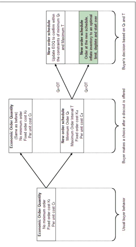
Buyer now faces a decision to make (see Figure 2-1). The o¤er has three parameters, the minimum quantity QT, the expiration date T , and the discount
rate r and the buyer will make his decision based on these three values. These parameters a¤ect the inventory level of the buyer and he needs to investigate what will happen if he chooses to utilize this o¤er. If QT is less than his demand
occurring during the time frame that the discount is available, i.e. DT , then he will utilize this discount without any further analysis as he needs to purchase more than QT to meet the demand from his customers. However if QT is greater than
DT, then the buyer is going to be increasing his inventory level if he chooses to use this o¤er, as extra supply will be purchased before the buyer needs to purchase again to meet customer demand.
The supplier has full knowledge of this situation as she is aware of the buyers past purchasing behavior. She could give an o¤er which would have a minium quantity less than the buyer’s DT but in this case the problem is trivial, the buyer will modify his purchase, either he would buy more than QT at the end of
each expiration date, or he would make purchases of size QT more frequently, while
enjoying the discounted prices. We will be investigating the interesting problem where QT is greater than DT: At this case, the buyer, if chooses to utilize the
o¤er, will be increasing his inventory inde…nitely and is expected to stop in‡ating his inventory at some point. This subcycle is called the "m subcycle" continuing
for m purchases. The buyer …rst makes a purchase of Q0 > QT at the list prices
and then makes a series of purchases greater than QT at the discounted prices.
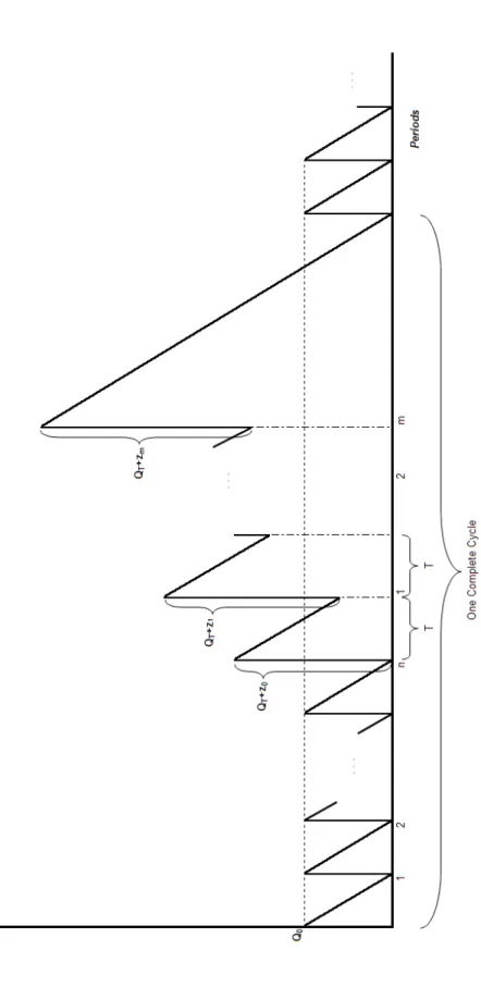
After the mth purchase, the buyer stops this cycle, makes his last purchase, where the order size is independent of QT, at the discount prices and starts meeting his
demand from his inventory until it is completely depleted; Figure 2-2 depicts the inventory level of the buyer through one full cycle.
Our problem de…nition states that there is an expiration date on the discount o¤er, T: During the construction of our cost functions we use this expiration date as the length of each period during the m subcycle. One might wonder if the buyer would purchase before this deal expires, i.e. the time between two orders could be less than T . However this would not be applicable to the case we are investigating; we know that QT > DT meaning that inventory purchased will not be depleted
by the end of the expiration date. This indicates that ordering before the deal expires would not be optimal to the buyer as he does not have any additional bene…ts from this behavior: He will be increasing his inventory, and his inventory carrying costs, earlier than he would need to if he chose to continue with the m subcycle. We will assume that the buyer would make his next purchase using the discount at the end of the expiration time, thus the time between two orders will be exactly T:
We are interested in …nding whether this cycle repeats itself, …rst the n subcycle then the m subcycle. Our aim is to see whether the n subcycle a¤ects the m subcycle, calculate the maximum inventory level that the buyer will be reaching and investigate under which conditions such a discount will be optimal to the
buyer. We will be looking at the total cost rate, calculated by total costs incurred through the complete cycle divided by the cycle length.
We introduce some notation below: Q0
0: Usual ordering quantity
QT: Discount eligible quantity
Qi: Order quantity in the cycle except last, i = 0 to m 1
Qm: Last order quantity
n: Number of times Q0
0 is ordered in the cycle
m: Number of orders of minimum size QT, m 1
T: Expiry date for the o¤er, length of each period during m subcycle
zi: Excess in Qi over QT such that Qi = QT + zi
D: Demand rate cl: Unit list price
cd: Unit discount price
Kl: List …xed ordering cost
Kd: Discount …xed ordering cost
h: Inventory holding cost per unit per unit of time
The objective from the buyer’s perspective is to obtain the optimal replenish-ment policy parameters (n ; Q0
rate. To this end, we will …rst derive the expressions for the operating charac-teristics of the system, and then derive the optimization results on the decision variables.
2.2
Operating Characteristics
In this section, we compute the operating characteristics of our model.
The cycle length, CL, consists of two segments: (i) the one corresponding to n many orders of the size Q0
0 during which no discount eligibility occurs and (ii)
the one corresponding to m orders during which discounts are taken into account, thus: CL = DnQ00+ mT + D1[mQT + m 1P i=0 zi mDT + Qm] = DnQ00+D1mQT + D1 m 1P i=0 zi+D1Qm (2.1)
The ordering cost per cycle, OC, consists of the …xed ordering costs associated with list and discount orders, hence:
OC = nKl+ Kl+ mKd
= (n + 1)Kl+ mKd
(2.2)
The holding cost per cycle, HC, is composed of the inventory related costs carried over the two subcycles. It is found by computing the area under the buyers inventory curve, see Figure 2-2, and is given by:
HC = 2DnhQ02 0 +f (QT+z0+QT+z0 DT ) 2 hT + ( 2(QT+z0 DT +QT+z1) DT 2 )hT + (2(2QT+z0+z1 2DT +QT+z2) DT 2 )hT + ::: + hT 2 (2[mQT + k 1P i=0 zi (k 1)DT ] DT )g + h 2D[mQT + m 1P i=0 zi mDT + Qm]2 HC = 2DnhQ02 0 +f m P k=1 2[kQT+ kP1 i=0 zi (k 1)DT ] DT 2 ghT + [mQT+ mP1 i=0 zi mDT +Qm]2h 2D (2.3) The purchase cost per cycle, PC, consists of expenses for purchasing units at the list and the discounted prices.
P C = nQ0
0cl+ cl(QT + z0) + cd m 1P
i=1
(QT + zi) + cdQm (2.4)
The total cost per cycle, CC, is given by CC=OC+HC+PC. Then the total cost rate, TC, can be written as follows:
T C = CC CL
= OC+HC+P CCL
(2.5)
2.3
Structural Results
In this section we obtain the analytical results on the structure of an optimal replenishment cycle for the buyer. We begin our results by showing that the buyer will not order more than QT during the m subcycle except for the last
Theorem 1 zi = 0 for all i = 0 to m 1:
Proof. Inventory position at the beginning of the mth period in the m subcy-cle depends on the cost values, since the inventory accumulated (either through acquisition in the previous periods or purchased at the beginning of the mth
pe-riod) will only have e¤ect on the future periods and is not dependent on the past periods. As we know that during the n-subcyle the inventory will be depleted by the nature of our setup, let us look at the inventory accumulated during the m-subcycle at the beginning of the mth period after the last purchase is made, ILm: ILm = m P i=0 Qi mDT = mQT + m 1P i=0 zi mDT + Qm
We know that orders are made every period until the mth period where the buyer decides to stop in‡ating his inventory, and purchases for the last time at the discounted prices and ends the cycle. Excess inventory purchased - purchases with order sizes larger than QT - during the m subcycle will be stored in the inventory,
only to be used at the mth period. We know that this is the case since we already
assume that QT > DT, hence a portion of that order will not be used, adding to
the extra inventory to be used after the last purchase of size Qm. However if that
excess is to be used at the mth period, the buyer has the opportunity to purchase
those items at the mth period, and he does not need to carry the inventory cost
for more than necessary. Thus it is obviously seen that if zi = 0 for all i = 0 to
m 1 then total inventory accumulated at the end of the (m 1)th period will be
that zi = 0 for all i = 0 to m 1:
Since we know that zi = 0 for all i = 0 to m 1 from Theorem 1, we will
rewrite the costs associated with the total cost rate, where for all i = 0 to m 1; Qi = QT. We leave Qm as is, it could have any value, as it is the last purchase at
the discounted prices, the buyer could order any quantity independent of QT. For
notational convenience, we will denote Q00, the order size during the n subcycle,
as Q0: CL = n DQ0+ mQT D + 1 DQm (2.6) OC = (n + 1)Kl+ mKd (2.7) HC = nh 2DQ 2 0 +f m P k=1 2[kQT (k 1)DT ] DT 2 ghT + [m(QT DT ) + Qm] 2 h 2D (2.8) P C = nQ0cl+ clQT + (m 1)cdQT + cdQm (2.9)
CC = (n + 1)Kl+ mKd+ 2DnhQ20+f m P k=1 2[kQT (k 1)DT ] DT 2 ghT + [m(QT DT ) + Qm]2 h2D + nQ0cl+ clQT + (m 1)cdQT + cdQm (2.10) We have computed our optimality condition and realized that the total cycle does not depend on n: Hence we know that the decision of the buyer does depend on his past purchases made in the n subcycle, but rather lies solely with the m subcycle.
Theorem 2 A mixed policy is not optimal in one cycle. Either the buyer will continue to purchase his EOQ or he will use the discounted schedule o¤ered by the supplier: Cycle will only use one of the two purchase o¤ers.
Proof. Employing the …rst order condition on n reveals that whichever cost rate is smallest in the subcycles will dominate. The detailed derivations are given in Appendix A.
Our initial setup was such that both subcycles will occur one after the other. However our …nding for n shows us that the n subcycle is not signi…cant in …nding the total cost rate of the complete cycle as the decision of using a discount o¤er does not lie with previous purchases but with the decision variables that are associated with the m subcycle. The proof of the theorem 2 is trivial in showing that past purchases do not a¤ect the future decisions. However, we have kept this part in this study, as it was the beginning motivation for our research. We wanted to be
able to see a cyclic motion, a cycle that is composed of two subcycles, basically a mixed order policy. We now see that this mixed policy does not occur, and either the EOQ policy or the discounted policy will be optimal to the buyer. The only instance where we could have an optimal mixed order policy will be if the supplier had an additional criterion on the buyer’s eligibility of the discount schedule; i.e. a de…nition of a "preferred customer". If this was the case, where the supplier made the discount o¤er only to customers she deemed "preferred" based on a criterion that included past purchases, than such a mixed policy might occur.
We have shown that our cycle composed of n and m subcycles do not repeat, and the decision of using the discounted ordering pattern depends on the m subcy-cle only. We will now proceed to formulate m subcysubcy-cle alone, and …nd m and Qm
through the total cost rate, i.e. total cost divided by cycle length. Our functions related to the total cost are the same as before, we only assume that n = 0:Let us look at the buyer’s cost functions once again.
Ordering cost per cycle is given by:
OC = Kl+ mKd (2.11)
Purchasing cost per cycle is given by:
Note that we have simpli…ed the expression for the holding cost per cycle, see Appendix A, proof of Theorem 3; then the holding cost is given by:
HC = m2( hT 2 QT + h 2DQ 2 T) + m( hT 2 QT + h DQmQT hQmT ) + h 2DQ 2 m (2.13)
Hence the cycle cost is:
CC = Kl+ mKd+ clQT + (m 1)cdQT + cdQm+ m2( hT2 QT +2Dh Q2T)+
m(hT2 QT +DhQmQT hQmT ) + 2Dh Q2m
(2.14) Finally the cycle length is given by:
CL = 1
DmQT + 1
DQm (2.15)
So the total cost rate is the ratio of the cycle cost to cycle length:
T C = 1 1 DmQT + 1 DQm [Kl+ mKd+ clQT + (m 1)cdQT + cdQm+ m2( hT 2 QT + h 2DQ 2 T) + m( hT 2 QT + h DQmQT hQmT ) + h 2DQ 2 m] (2.16)
Before investigating the optimal values of m and Qm, let us look at the
con-vexity of the buyer’s total cost rate.
Theorem 3 For all m 1; TC is quasi-convex in Qm: Furthermore, for all
Qm 0; TC is quasi-convex in m:
Proof. This result follows from computing the second derivatives of the cycle cost and the cycle length with respect to Qm and m. We show that cycle cost is
convex in Qm and cycle length is concave in Qm for m 1;for the quasi-convexity
of the cost rate in Qm:Similarly we show that cycle cost is convex in m and cycle
length is concave in m for Qm 0; see appendix A for the proof.
The quasi-convexity of the buyer’s total cost rate in m and Qm indicates that
the total cost rate function is unimodal, we could …nd the extrema for m and Qm
for the total cost rate. To …nd the these values we will look at the …rst order condition of the total cost rate. We simplify the …rst order condition as follows: Assume that A and B are functions in x, then the …rst order condition will be
@ @x( A B) = 0: @ @x( A B) = 1 B2( @A @xB A @B @x) = 0 @A @xB 1 B2 A@B@xB12 = 0 @A @x 1 B = A @B @x 1 B2 @A @x = A @B @x 1 B
@A @x @B @x = A B (2.17)
We will be using the above result in …nding the extrema of the total cost rate. We …rst investigate the extrema of Qm;which we denote by
^
Qm:
Lemma 1 For any m > 1, Q^m is equal to the single positive root to the equation:
h 2DQ 2 m+mDhQTQm Kl mKd clQT+cdQT m 2 hT 2 QT+m 2 h 2DQ 2 T mhT2 QT = 0
if it exists; otherwise, Qm is zero.
Proof. Follows from the …rst order condition, see Appendix A.
We have found theQ^mfor any value of m: We then set the …rst order equations
with respect to m and Qm to each other and …nd another result.
Lemma 2 When m = m,^ Q^m is also given by the equation hT1 Kd+12QT.
Proof. Follows from equalizing the …rst order condition of the buyer’s cost rate with respect to m and Qm, see Appendix A.
As we have found Qm for any positive m, we will now compute m: But note
that m is integer valued. Therefore we could …nd the optimal m through the …rst di¤erence condition; m is the minimum m such that:
T C(m + 1) T C(m) 0 (2.18)
Lemma 3 When Qm = hT1 Kd + 12QT, ^
m is given by unique positive root that solves the following:
m2( hT 2 QT + h 2DQ 2 T) + m( 1 DTKdQT + h 2DQ 2 T Kd hT2 QT) + 2DT hT1 Kd2 + 1 2T DQTKd+ cdQT clQT Kl+ h 8DQ 2 T = 0
Proof. Proof rests on computing the …rst order condition of the buyer’s total cost rate with respect to m when Qm = hT1 Kd+12QT: See Appendix A for details.
Theorem 3 does not prove thatm^ will always have a positive root, it only shows that b p2ab2 4ac will always be negative when QT > DT: Positivity of b+
p b2 4ac
2a
depends on the coe¢ cients of the quadratic equation, i.e. the costs, quantities and the discounts associated with any given problem, so we could possibly …nd a negative value for m. This would be meaningless, in such a case, a non-optimal but positive m could be calculated where the buyer still has incentive to utilize the given discount o¤er. We will not look further into this detail, during our numerical study any negative m found will be discarded and those cases will not be used.
Following Theorem 2, note that Qm is independent of the number of orders
placed before within a cycle. This does not imply that Qm in general, for any m,
does not depend on m: But rather the optimal Qm in an optimal cycle with m
does not. Remark:
There are two cases that need to be answered to show that when the m subcycle ends, the discount o¤er will no longer be available to the buyer.
1. Qm QT :If Qm is greater than or equal to QT then, as QT is strictly greater
than DT; we know that when the buyer’s inventory depletes the discount o¤er that is presented due to the order Qm QT will be withdrawn. This is
due to the fact that the expiry date would have passed, so the buyer could only restart the cycle at this point.
2. Qm < QT :If Qm is less than QT, the buyer’s inventory could deplete before
or after the expiry date, this depends on previous inventory accumulated by the buyer. However in this case, as the last purchase made does not meet the minimum order criteria, the buyer will not be o¤ered a discount, and independent of the time that the new order comes, he will need to restart the cycle.
The above results are based on the identi…cation of the extrema of T C. Next, we examine the convexity properties of the total cost rate. We will be looking at the positivity of the second derivative of the buyer’s total cost rate.
Theorem 4 For any Qm set at [hT1 Kd+12QT], the buyer’s total cost rate function
is convex in m if: Q2 TH2Dhm + QTH22h + QTH1D2 + Q2T H1 H2 2 D2m > QTH2hT m + H22hT D + 2H2H3+ QTH3D2m where H1 = 2DhT1 2K 2 d+ 8Dh Q 2 T + 2T D1 KdQT + clQT + cd 1 hTKd 1 2cdQT + Kl H2 = 1 Kd+ 1 QT
H3 = DT1 KdQT + 2Dh Q2T + cdQT
Proof. The proof follows from calculation of the Hessian of the total cost rate as given in Appendix A.
Theorem 4 provides the necessary condition for the convexity of the buyer’s total cost rate. Below result provides the su¢ cient condition for this convexity.
Corollary 1 For any Qm set at [hT1 Kd+12QT], it su¢ ces to have Kl> 2Dh [hT1 Kd+ 1
2QT]
2 for T C to be convex in m.
Proof. Follow immediately by considering individual terms in Theorem 4 separately, as given in Appendix A.
We can show that the …rst and the second terms on the left hand side of the inequality in Theorem 4 are greater than their corresponding terms on the right hand side, as long as QT > DT. However, we can not say the same for the third
and the fourth terms. As seen through Corollary 1, one could identify cases where the convexity does not hold. However we are certain that the convexity holds for out intents and purposes, as we have performed extensive numerical checks. During the numerical analysis that we have performed, none of the experiment instances considered violated the necessary condition for convexity.
We have also looked at cases where the above equation might not hold, and our analysis indicate that this equation holds as long as we don’t have a small discount rate with a high QT with respect to T and the demand rate. If the
increases his inventory drastically, i.e. QT is very large compared to DT , then
convexity might not hold. We have not done an in depth analysis where we could identify cuto¤ points or conditions where this would occur, but we can argue that under such circumstances the buyer would not be interested in using the discount o¤er. Hence, we can conclude that for our purposes the payo¤ function is convex. We now know the su¢ cient condition for the convexity of the buyer’s total cost rate and moreover we know the extrema of the total cost rate in m and Qm:Then
we could write the following Theorem 5 about the optimality of the total cost rate function
Theorem 5 For any Qm = hT1 Kd+ 12QT and m given by the quadratic equation
given in Lemma 3; if the su¢ ciency condition given by Corollary 1 holds, then:
1. Qm = hT1 Kd+ 1 2QT 2. m is either (a) 1, or (b) dme, or (c) bmc.
when dxe and bxc denote the ceiling and ‡oor functions, respectively.
Proof. We have shown that the buyer’s total cost rate is quasi-convex in Qm
and m indicating that this function is unimodal. We have then found the values of Qm and m that minimize the total cost rate function of the buyer. We have also
given the necessary and su¢ cient conditions for the convexity of the buyer’s total cost rate. As we know the unimodality, we know that the optimal values of Qm and
m will either be given by the extrema that we have computed or the boundary conditions that are found. If the value of m exists when Qm = hT1 Kd + 12QT
then we know that there exists an optimal discount o¤er for the buyer given by the couplet (Qm; m ) where Qm = hT1 Kd+
1
2QT and m is given by one of the
following, whichever provides a smaller TC, 1; dme or bmc:
We have identi…ed the decision variables of the buyer’s total cost rate. By computing Qm and m the buyer enables to …nd the optimal values of his decision
variables, and make a comparison of the discounted schedule with his EOQ order. He can then decide whether he will utilize the discount o¤er or not.
CHAPTER 3
SUPPLIER’S CASE
We have so far concentrated on the buyer and his decisions and have assumed a discount schedule o¤ered by the supplier without investigating her decisions and cost functions. In this section we will look at the supplier and her possible motives to provide such a discount.
We know that the o¤ered schedule does not alter the total quantity that the buyer purchases over time. The supplier is not selling more units and because of the discount, her revenues are decreasing. Even under this condition, there could be motives for the supplier to o¤er this discounted schedule. We know that such discounts alter the buyer’s purchasing frequency. Over the length of a cycle we know that if he orders his EOQ, the buyer’s order frequency will be uniformly distributed but if he follows the discounted schedule, he will be purchasing more frequently at the beginning of the cycle and there would be a longer period at the end of the cycle where he does not make any purchases. This would a¤ect the
supplier’s in‡ow of cash, as in an EOQ schedule her cash‡ows would be uniformly distributed whereas in the discounted schedule she will be receiving the total payments in a shorter amount of time. Due to this case we can safely assume that if the supplier is in need of cash earlier, she might have incentives to sell more earlier to feed this need. We will not look into this case in this thesis, as it is out of its scope, but this case remains an important point as an incentive for the supplier.
The second incentive would be the holding costs that the supplier incurs. Sup-plier, through the use of this discount, is minimizing her inventory related costs. This approach has been previously used by Wang (2002), Dara and Srinkanth (1987) and Lal and Staelin (1984). We do not consider the supplier’s inventory replenishment policies, but basically assume that she has inventory stored, and she is meeting the demand of the buyer from this stock. As the buyer is o¤ered to in‡ate his orders, the inventory held by the supplier is transferred to the buyer before the buyer needs that stock. This policy enables the supplier to save on her inventory related costs, and through these additional gains she is able to o¤er a discount to the buyer.
We propose that the decision criteria for the supplier’s decision is based on her holding cost ratio to the buyer’s holding cost. As the supplier is going to receive a smaller total payment, she needs to break even through the transferred costs. We know that the buyer is also paying extra in holding costs. Then the ratio of these extra holding costs to the supplier’s loss is the same as the ratio of the buyer’s holding cost to the supplier’s holding cost.
We will …rst look at the supplier’s pro…t under the two ordering schemes. Let SRE denote the supplier’s pro…t when buyer orders his EOQ per unit time and
let SRD denote the supplier’s pro…t when buyer orders discounted schedule per
unit time.
Let us look at the supplier’s pro…t under the EOQ policy, which is given by the sum of the revenue from sales and gains from the transfer of inventory related costs:
SRE = Dcl+
Q0
2 h (3.1)
Let us look at the supplier’s pro…t under the discount policy, which is given by the sum of the revenue from sales under discount and gains from the transfer of inventory related costs, minus the lost revenue from …xed cost:
SRD = Dcd+ CL1 [m2( hT2 QT +2Dh Q2T) + m( hT 2 QT + h DQmQT hQmT ) + h 2DQ 2 m] 1 CLm(Kl Kd) (3.2) where the cycle length, CL, is equal to 1
DmQT + 1 DQm:
We know that the supplier will only o¤er a discount if she is not worse o¤. Let us look at the supplier’s break-even point, the supplier will o¤er a discount if:
If the above condition holds, then the supplier, for a given discount schedule, will be pro…ting. If, at the same time, this discount schedule is pro…table to the buyer as well, then both parties will have a motivation to use the discount policy. Now let us look at the inventory costs of the buyer; we denote the buyer’s inventory cost following EOQ schedule as HCBEOQ, the buyer’s inventory cost
following discounted schedule as HCBD;and the supplier’s unit-time holding cost
as h0:
Buyer’s inventory cost rate following EOQ:
HCBEOQ=
Q0
2 h (3.4)
Buyer’s inventory cost rate following discounted schedule:
HCBD = [m2( hT 2 QT+ h 2DQ 2 T)+m(hT2 QT+ h DQmQT hQmT )+ h 2DQ 2 m] 1 DmQT+ 1 DQm (3.5)
Buyer’s additional cost on inventory - as QT > DT - is equal to HCBD
HCBEOQ: This cost is also equal to the inventory cost that is not paid by the
supplier, as this is the quantity that the supplier transferred to the buyer through the discount o¤er. If the supplier is pro…ting, i.e. SRD SRE 0, then we could
say that:
(SRD SRE) h = h0 (HCBD HCBEOQ)
h0
h =
SRD SRE
HCBD HCBEOQ
(3.6)
This ratio gives us a decision criterion as it acts as a break-even point for any given discount o¤er. If, for a given discount o¤ering which bene…ts the buyer, the actual holding cost ratio of the supplier to the buyer is higher than the calculated percentage then the supplier will also bene…t from the discount. The breakeven point gives the supplier the criterion to o¤er a discount that bene…ts both parties.
CHAPTER 4
NUMERICAL ANALYSIS
Our theoretical …ndings have given us the basic rules in determining our system. We will now undertake a numerical study to further investigate the e¤ects of our discount schedule.
Our study will be comparing an EOQ case versus a schedule with expiring dis-counts. Our initial problem setting de…ned a cycle as a combination of two distinct schedules. First buyer purchases a number of EOQ orders and then purchases the increased orders. As we have previously shown, this does not happen; the EOQ orders do not have any impact on the later decisions faced by the buyer when a discounted schedule is o¤ered. Hence the buyer will either choose to continue his EOQ schedule or will switch to an increased order that will enlarge his inventory until it is no longer pro…table to do so where he will quit purchasing until his inventory depletes. Our numerical study will investigate this case.
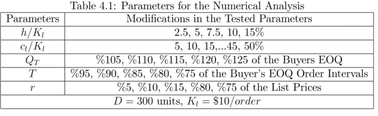
investigation. Each of these reference points is termed a "case" for convenience in later discussions. Each case had a demand of 300 units per month and an ordering cost of $10 per order. Five di¤erent holding costs used, varied as 2.5, 5, 7.5, 10, and 15 percent of the ordering cost. Similarly ten di¤erent unit variable costs are used from 5% to 50%, increasing with 5% increments, again as a percent of the ordering cost.
The reason behind using a constant ordering cost and holding cost represented as a percentage of the ordering cost is as follows: The order cost, as it is incurred every order regardless of order size, has a big impact on the frequency of orders. If the order cost to holding cost ratio is high, the calculated EOQ will be larger than it would be in the opposite case where such a ratio has a lower value. So varying holding cost with respect to a constant order cost captures this phenomena. If we look at the variable cost, similarly as the as aforementioned argument, it could be argued that order cost to variable cost ratio might change the ensuing EOQ size to change.
Summarizing, we had a total of 50 cases, as we had 5 di¤erent holding cost and 10 di¤erent variable costs a total of 50 combinations, to be used as benchmarks when we concluded our numerical analysis. For each case we have calculated the economic order quantity and the time between two orders along with a total cost per month which is a linear term; total cost per order projected over a month.
Each of our 50 cases were subjected to 125 di¤erent "o¤erings". For conve-nience we de…ne an o¤ering as a speci…c instant of a given discount percentage on the order and variable costs, an order interval T , and a minimum purchase
amount Qt. Each of these variables were changed 5 times hence a total of 125
combinations for each case.
The discount percentage, r, r = 1 cd=cl = 1 Kd=Kl; is used to …nd Kd and
cdfrom Kland cl, varying from a 5% discount to 25% discount in equal increments
of 5%. Similarly Qt is found using the order sizes calculated for each case, i.e. the
economic order quantities, increased by 5% to 25% in equal increments of 5%. For the order interval T we have shortened the order intervals calculated for the cases by 5% to 25% in equal increments of 5%. See Table 4.1 for a summary of the parameters used in the numerical analysis.
We have investigated a total of 6250 o¤erings. For each o¤ering Qm and m
are …rst found. Then according to our problem setting, m orders of Qt is made
followed by the last order Qm. First Qtis purchased by the buyer at the list prices,
and following orders are purchased at the discounted costs. Total cost per cycle is calculated where a cycle de…ned as the total time between the time that the …rst order is made until all of the inventory is depleted after the last order Qm is
made. Then this cost is linearly converted to a per month cost to be compared against the original case.
Note that m could be found to be negative, as this is meaningless we will not take these o¤erings into consideration. Moreover it should be noted that we have used real numbered values for each case and o¤ering, hence ordering a fraction of a unit is allowed and similarly m takes on real values i.e. the buyer could order a real valued number of times, this shortcoming will be addressed later.
Table 4.1: Parameters for the Numerical Analysis Parameters Modi…cations in the Tested Parameters
h=Kl 2.5, 5, 7.5, 10, 15%
cl=Kl 5, 10, 15,...45, 50%
QT %105, %110, %115, %120, %125 of the Buyers EOQ
T %95, %90, %85, %80, %75 of the Buyer’s EOQ Order Intervals r %5, %10, %15, %80, %75 of the List Prices
D = 300 units, Kl= $10=order
4.1
Results
We will investigate our results in three sections: (i) Sensitivity,(ii) Impact of real value approximation, and (iii) Advantages to the seller. Note that our results hold for the su¢ cient condition for the convexity that we have discussed earlier.
4.1.1
Sensitivity
We will examine the sensitivity of the optimal policy parameter values with the First let us look at the relationship between T , QT, m, and r. Note that in
our previous discussions, we used a di¤erent notation for the list and discounted prices, however, they could have easily been replaced by multiplying list prices by a discount percentage where r = 1 cd=cl = 1 Kd=Kl:
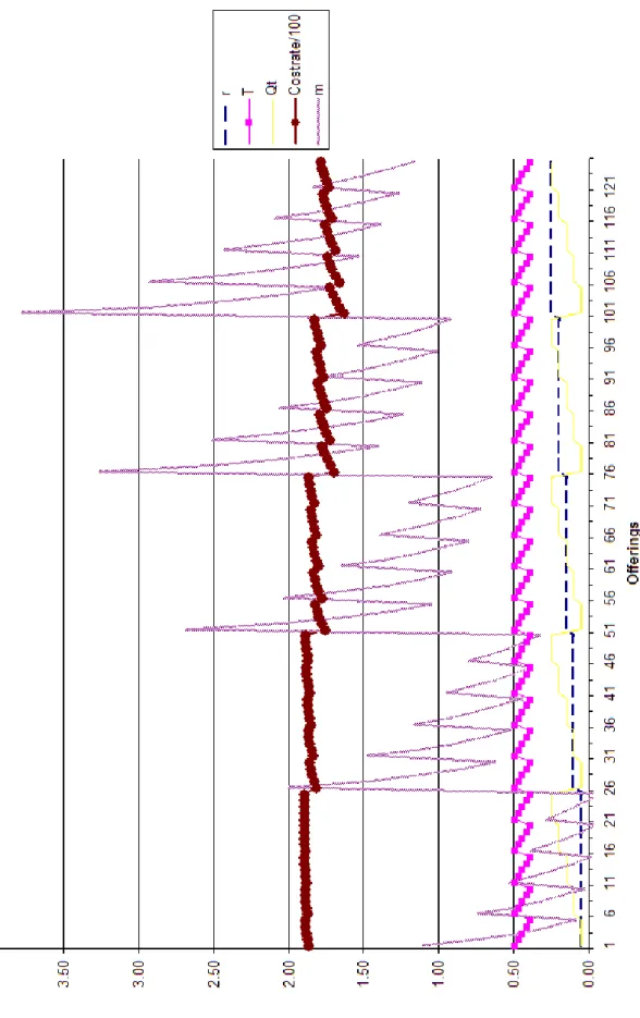
We …nd that T and r have a direct relationship with m - as they are increased malso increases - whereas QT has an inverse relationship with m. We also observe
that m and the total cost rate have a direct relationship and increasing m decreases the total bene…ts (since total cost rate increases). The reader is referred to Figure 4-1 for the above conclusions.
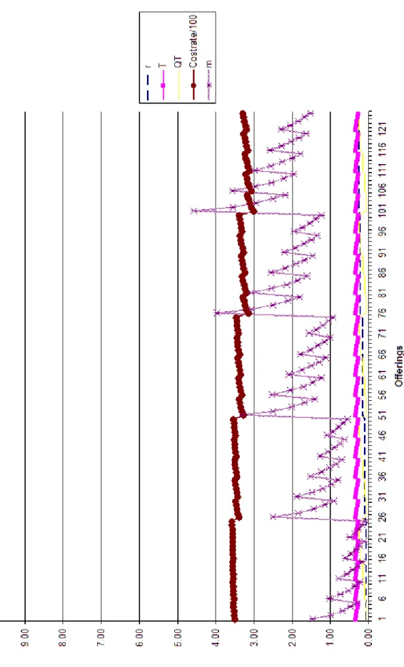
Figure 4-1: Changes in T, Qt, m and Discount Percentage and their relationship with Total Cost Rate for Case 1
300, order cost $10, variable cost $0.5, holding cost $0.25, and economic order quantity 155 units, and the time between two EOQ orders at 0.516 months. This graph is representative among all cases, we nevertheless have included sample graphs for cases 7, 15, and 32 for comparisons as well.
These …ndings are very logical, as m increases, the cycle length increases and the buyer is forced to keep additional inventory for a longer period of time hence the total cost increase, thus higher values of m is not bene…cial. As T increases, m also increases, this could be attributed to the fact that as T increases, the time between two orders becomes closer in value to the order interval during the EOQ pattern. Increases in QT decreases m, which is due to the fact that increasing QT
forces the buyer to keep a larger inventory, hence his inventory level increases to his optimal maximum quicker, thus m decreases. Finally discount percentage and m has a direct relationship, indicating that higher discounts make it possible for the buyer to stay in the cycle for a longer period of time. Table 4.2 summarizes the above …ndings.
Observing the di¤erences between cases, we see that increasing holding cost increases the total cost rate, decreasing the savings, which is expected. Another observation is that as the variable cost percentage (cl=Kl) increases the number
cases that show savings increase. Variable cost percentage is the cost per item that is calculated as a percentage of the …xed order cost. As we increase this percentage, the e¤ect of the …xed cost decreases, and the cycle cost becomes less sensitive to the …xed cost since the overall number of orders has limited a¤ect on the cycle cost. Some obvious results also were observed, we have a smaller number
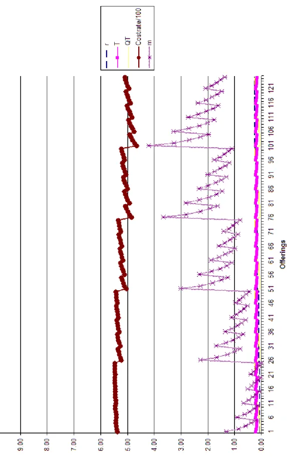
Figure 4-2: Changes in T, Qt, m and Discount Percentage and their relationship with Total Cost Rate for Case 7
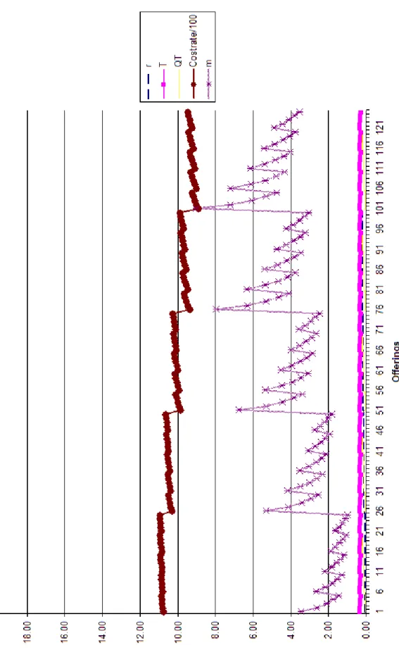
Figure 4-3: Changes in T, Qt, m and Discount Percentage and their relationship with Total Cost Rate for Case 15
Figure 4-4: Changes in T, Qt, m and Discount Percentage and their relationship with Total Cost Rate for Case 32
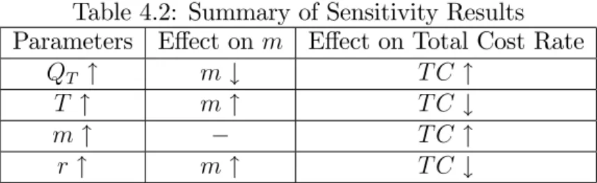
Table 4.2: Summary of Sensitivity Results Parameters E¤ect on m E¤ect on Total Cost Rate
QT " m# T C "
T " m" T C #
m " T C "
r" m" T C #
of o¤erings that show savings with increased QT, and we have a higher number of
o¤erings showing savings with higher discount percentages.
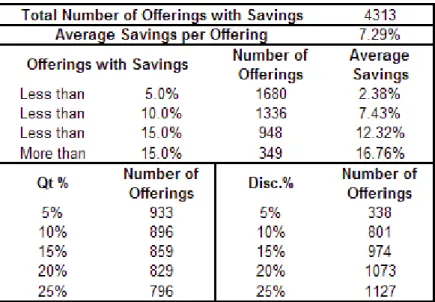
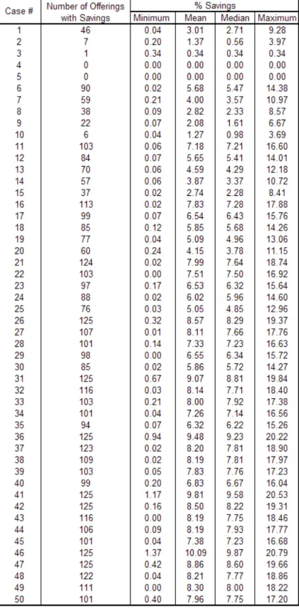
Overall, of the 6250 o¤erings, 4313 of those showed savings. Table 4.3 contains descriptive statistics cases when m was a real number. Table 4.4 contains the number of discount o¤erings that were pro…table for each case and statistical information on the savings percentages. Average savings were 7.29%, and were as high as 20.79%. We see that the highest concentration of o¤erings showed less than 5% savings, however almost 6% of all o¤erings had more than 15% savings. We also see that increasing QT had a negative e¤ect on the number of o¤erings
with savings while the discount rate r had a positive e¤ect, almost all of the o¤erings with 25% discount (1127/1250) showed positive savings for the buyer. Of all cases, only cases 4 and 5 did not have any o¤erings with a positive discount, these two cases had high holding costs (h=Kl = 0:1and 0:15 respectively) and low
unit variable cost ratios with the …xed cost (cl=Kl= 0:05 for both).
4.1.2
Impact of real value approximation
Note that we have used real valued m’s for this analysis. However, we have previously shown that total cost rate function is convex when around the optimal
Table 4.3: Descriptive Statistics of the results when m is real valued
m hence the optimal m provides for a minimum for the total cost rate. This allows us to compute the optimal m and then round it to the 2 nearest integers, one of which will be the unique integer that minimizes the total cost rate, and compute the cycle cost using these rounded-up and rounded-down m values. Then the decision is to basically use the m which provides the lower total cost rate.
This was investigated during our numerical analysis. We see that the total cost rate that is calculated using the optimal m value creates a lower bound for the total cost rate calculated with rounded up and down values of m. We also noted that the overall trend of the total cost rate is similar in all three calculations, except for certain o¤erings where m was not rounded down (if m < 1 then m = 1) to be able to provide meaningful results. See Figure 4-5.
We found that when m is rounded down the number of discount o¤erings with savings dropped to 4251 and when m is rounded up the number of o¤erings with
Figure 4-5: Total cost rate calculated for real valued m, rounded-up m and rounded-down m and the EOQ
savings was 4274. As we know, if m is optimal and real valued these numbers would have been 4313. Sensitivity statistics are provided in the Tables 4.5 and 4.6.
We have also run our analysis for the optimal value of the integer m. We have calculated both instances of the total cost rate when m was rounded, and selected the one with a better result for the total cost rate. In this case we see that the total number of discount o¤erings with savings for the buyer was 4296 with an average savings per discount o¤ering of 7.31%. Note that mean savings are higher in the cases when m is rounded; this is due to the fact that discount o¤erings with small savings, where the calculated total cost rate is very close to the EOQ cost, are eliminated during rounding, hence the mean increases. Table 4.7 has the sensitivity information for the analysis when we looked at the optimal integer value of m:
4.1.3
Advantages of the Seller
We have calculated the holding cost ratios in our numerical analysis, Figure 4-6 presents this ratio for o¤erings made in Case 1 - note that the o¤erings where buyer does not make a pro…t has no calculation of the ratio. Here we see that as discount rates increase, the ratio increases, which is logical because the increase in discount rate decreases supplier revenues. On the contrary as T decreases, we see that the ratio decreases; making it more pro…table for the supplier, which coincides with our previous result where decreases in T made buyer worse o¤. QT has a
Table 4.8: Results on the holding cost ratios of the seller to the buyer
similar e¤ect to the seller, contrary to the buyer, increases in QT is pro…table to
the supplier. We have calculated the holding cost ratios for all discount o¤erings where the buyer was saving, Table 4.8 contains the descriptive statistics. Note that 1574 out of the 4313 discount o¤erings which showed savings has a calculated ratio less than 100%. In the literature, it is assumed that the supplier will have a smaller holding cost rate than the buyer. If this assumption holds, 25.2% of all discount o¤erings or 36.5% of the discount o¤erings that had savings for the buyer, will be pro…table to the supplier as well.
We have conducted other studies for additional results. Note that we have previously remarked that the buyer will not be able to continue his cycle when his inventory depleted following his Qm purchase. We have con…rmed this result
during our numerical study. Even though there were cases when Qm was less than
QT; the inventory accumulated after the Qm purchase have always depleted after
the expiry date T: The time it took to deplete ranged from 0:03 to 1:58 time units (in our case months) after T time units have passed.
We have also computed our results for cases where Kd = Kl to be able to
Figure 4-6: Ratio of the holding cost of the supplier to the holding cost of the buyer, computed for o¤erings in Case 1
the number of o¤erings where savings occurred for the buyer was smaller, 4187 o¤erings vs. 4313 o¤erings with order cost discounted.
CHAPTER 5
CONCLUSIONS AND FUTURE
WORK
We have looked at a single buyer-single supplier system under an EOQ setting with quantity discounts and expiry dates. We obtained the optimal replenishment policy parameters for the buyer. We have also extended our research discussing the supplier’s motivation and decisions in some detail and with a numerical example to show that this model captures our intuitive results.
The contribution of this study to the current stream of literature lies with the expiry dates. Expiring quantity discounts have not been studied within the literature and we provide a basic set of decisions that could be further investigated by academicians in detail.
Our research has shortcomings as well, basically due to our starting assump-tions. We assumed the demand that the buyer faces does not change with his
supply, which could be restrictive however one should consider that if the demand rate increases, the buyer will be better o¤ than what we have provided here - as it would be unrealistic to assume that his demand will decrease due to increase in supply.
Another shortcoming for our research is that we use the EOQ policy to compare our results, instead of a stochastic system. Although it has been shown in the previous literature that the EOQ model is a good approximation of the real world scenarios, possible future work on this area might be including stochastic elements to this model.
We also believe that the supplier’s case should be investigated more in detail as it was an extension for us, we have not looked at this case in the required detail. We have not solved for the supplier’s decisions QT, T , and r, but only
provided some insight for her decision based on the holding cost ratio of the supplier to her customer’s. This insight does not take into consideration of the supplier’s inventory replenishment policy and assumes that the supplier’s ordering (or producing) frequency would not be changed when o¤ering such a discount schedule. This simpli…cation, as it is suboptimal, should be tackled in future research.
Bibliography
Benton, W.C., Park, S. 1996. "A Classi…cation of Literature on Determining the Lot Size under Quantity Discounts," European Journal of Operations Research 92(2):219-238.
Chen, F. 1999. "Decentralized Supply Chains Subject to Information Delays," Management Science 45(8):1076-1090.
Dana, Z.M., Srinkanth K.N. 1987. "Pricing Policies for Quantity Discounts," Man-agement Science 33(10):1247-1252
Dolan, R.J. 1987. "Quantity Discounts: Managerial Issues and Research Oppor-tunities," Marketing Science 6(1):1-22.
Joglekar, P.N. 1988. "Comments on a Quantity Discount Pricing Model to Increase Vendor Pro…ts," Management Science 34(11):1391-1398.
Krishna, A., Zhang, J.Z. 1999. "Short- or Long-Duration Coupons: The E¤ect of the Expiration Date on the Pro…tability of Coupon Promotions" Management Science 45(8):1041-1056.
Kohli, R., Park, H. 1989. "A Cooperative Game Theory Model of Quantity Dis-counts," Management Science 35(6):693-707.
Lal, R., Staelin, R. 1984. "An Approach for Developing an Optimal Discount Pricing Policy," Management Science 35(6):693-707.
Lee, H.L., Rosenblatt, M.J. 1986. "A Generalized Quantity Discount Pricing Model to Increase Supplier’s Pro…ts," Management Science 32(9):1177-1185.
Matta, K.F. 1994. "Ordering Policies for the Cyclical Replenishment Problem Given Lead Time-Dependent Discounts," European Journal of Operations Re-search, 73(3): 465-471.
Monahan, J.P. 1984. "A Quantity Pricing Model to Increase Vendor Pro…ts," Management Science 35(6):720-726.
Monahan, J.P. 1988. "Reply: On "Comments on a Quantity Discount Pricing Model to Increase Vendor Pro…ts"," Management Science 34(11):1398-1400.
Munson, C.L., Rosenblatt, M.J. 1998. "Theories and Realities of Quantity Dis-counts: An Exploratory Study," Production and Operations Management 7(4):352-369.
Parlar, M., Wang, Q. 1994 "Discounting decisions in a supplier-buyer relationship with a linear buyer’s demand," IIE Transactions 26(2):34-41.
Sahin, F., Robinson, P.E. 2002. "Flow Coordination and Information Sharing in Supply Chains: Review, Implications and Directions for Future Research," Decision Science 33(4):505-536.
Sirias, D., Mehra, S. 2005. "Quantity Discount versus Lead Time-Dependent Dis-count in an Inter-Organizational Supply Chain," International Journal of Pro-duction Research 43(16):3481-3496.
Wang, Q. 2002. "Determination of Suppliers’Optimal Quantity Discount Sched-ules with Heterogeneous Buyers," Naval Research Logistics 49(1):46-59.
Weng, K. 1995. "Channel Coordination and Quantity Discounts," Management Science 41(9):1509-1522.
Whang, S. 1993. "Analysis of Inter-Organizational Information Sharing," Journal of Organizational Computing 3(3):257-277.
Appendix A
Proofs
A.1
Proof of Theorem 2
Proof. 2 CC = (n + 1)Kl+ mKd+2DnhQ20+f m P k=1 2[kQT (k 1)DT ] DT 2 ghT + [m(QT DT ) + Qm]2 h2D + nQ0cl+ clQT + (m 1)cdQT + cdQm CL = DnQ0+ D1mQT + D1Qm
Our optimality condition is: @CC@n @CL @n = CC CL @CC @n = Kl+ h 2DQ 2 0+ Q0cl @CL @n = 1 DQ0 @CC @n @CL @n = DKl Q0 + h 2Q0+ clD Then,
DKl Q0 + h 2Q0+ clD = 1 n DQ0+ 1 DmQT+D1Qm [(n+1)Kl+mKd+2DnhQ20+f m P k=1 2[kQT (k 1)DT ] DT 2 ghT +[m(QT DT ) + Qm]2 h2D + nQ0cl+ clQT + (m 1)cdQT + cdQm]
Let us look at the left-hand side: LHS = (DKl Q0 + h 2Q0+ clD)( n DQ0+ 1 DmQT + 1 DQm) =) (DKl Q0 + h 2Q0+ clD)( 1 DmQT + 1 DQm) + DKl Q0 n DQ0+ h 2Q0 n DQ0+ clD n DQ0 =) (DKl Q0 + h 2Q0+ clD)( 1 DmQT + 1 DQm) + Kln + nh 2DQ 2 0+ clnQ0
Now let us look at the right-hand side: RHS = (n + 1)Kl + mKd+ 2DnhQ20 +f m P k=1 2[kQT (k 1)DT ] DT 2 ghT + [m(QT DT ) + Qm]2 h2D + nQ0cl+ clQT + (m 1)cdQT + cdQm =) nKl+2DnhQ20+ nQ0cl+ Kl+ mKd+f m P k=1 2[kQT (k 1)DT ] DT 2 ghT + [m(QT DT ) + Qm]2 h2D + clQT + (m 1)cdQT + cdQm Then LHS=RHS (DKl Q0 + h 2Q0+ clD)( 1 DmQT + 1 DQm) + Kln + nh 2DQ 2 0 + clnQ0 = nKl+ 2DnhQ20+ nQ0cl+ Kl+ mKd+f m P k=1 2[kQT (k 1)DT ] DT 2 ghT + [m(QT DT ) + Qm] 2 h 2D+ clQT+ (m 1)cdQT + cdQm =) (DKl Q0 + h 2Q0+clD)( 1 DmQT+ 1 DQm) = Kl+mKd+f m P k=1 2[kQT (k 1)DT ] DT 2 ghT + [m(QT DT ) + Qm]2 h2D + clQT + (m 1)cdQT + cdQm
We see that the terms that include n has cancelled out of the equation. This means that the decision of the buyer to accept a discounted o¤er does not depend
on his past purchases but rather at the discounted schedule. This also means that, if the buyer …nds the discounted schedule to be pro…table, he will switch to this schedule as long as it is available, indicating that he will either repeat his undiscounted cycle or the discounted cycle. Our de…nition of one complete cycle will not happen.
A.2
Proof of Theorem 3
Proof. 3
We will now show the quasi-convexity properties of the total cost rate in m and Qm:However, let us further simplify the cycle cost before we show our results
on the convexity. CC = Kl+ mKd+ clQT+ (m 1)cdQT + cdQm+f m P k=1 2[kQT (k 1)DT ] DT 2 ghT + [m(QT DT ) + Qm]2 h2D
Let us look at the holding cost component of the cycle cost, CC. HC = f m P k=1 2[kQT (k 1)DT ] DT 2 ghT + [m(QT DT ) + Qm] 2 h 2D =) hT m P k=1 2kQT 2 hT m P k=1 2(k 1)DT 2 hT m P k=1 DT 2 + [m(QT DT ) + Qm] 2 h 2D =) hT QT (m+1)m 2 hT m P k=1 kDT + hT m P k=1 DT hT2 m P k=1 DT + [m(QT DT ) + Qm]2 h2D =) hT QT(m+1)m2 hT DT(m+1)m2 + hT2 m P k=1 DT + [m(QT DT ) + Qm]2 h2D =) hT(m+1)m2 (QT DT ) + hT mDT2 + [m(QT DT ) + Qm]2 h2D
=) hT2 (m2 + m)(Q T DT ) + hT mDT2 + [m2(Q2T 2QTDT + D2T2) + Q2m+ 2m(QT DT )Qm]2Dh =) hT2 (m2+ m)QT hT2 (m2+ m)DT + hT mDT2 + m2 h2DQ2T m2 h2D2QTDT + m2 h 2DD 2T2+ h 2DQ 2 m+ 2m h 2DQmQT 2m h 2DQmDT =) hT2 QTm2+hT2 QTm hT2 DT m2 hT2 DT m+hT mDT2 +m2 h2DQ2T m2hQTT + m2 h 2DT 2+ h 2DQ 2 m+ mDhQmQT mhQmT =) hT2 QTm + m2 h2DQ2T 1 2m 2hQ TT + 2Dh Q2m+ mDhQmQT mhQmT =) m2( hT 2 QT + h 2DQ 2 T) + m( hT 2 QT + h DQmQT hQmT ) + h 2DQ 2 m
Then the cycle cost is equal to:
CC = Kl + mKd+ clQT + (m 1)cdQT + cdQm + m2( hT2 QT + 2Dh Q2T) +
m(hT2 QT +DhQmQT hQmT ) + 2Dh Q2m
Now let us look at the second derivatives of the cycle cost and the cycle length with respect to Qm: CC = Kl + mKd+ clQT + (m 1)cdQT + cdQm + m2( hT2 QT + 2Dh Q2T) + m(hT2 QT +DhQmQT hQmT ) + 2Dh Q2m @CC @Qm = cd+ m h DQT mhT + 2 h 2DQm @2CC @Q2 m = h D CL = D1mQT + D1Qm @CL @Qm = 1 D @2CL @Q2 m = 0