M. E. Kuhl, N. M. Steiger, F. B. Armstrong, and J. A. Joines, eds.
ABSTRACT
A simulation based learning mechanism is proposed in this study. The system learns in the manufacturing environment by constructing a learning tree and selects a dispatching rule from the tree for each scheduling period. The system utilizes the process control charts to monitor the perform-ance of the learning tree which is automatically updated whenever necessary. Therefore, the system adapts itself for the changes in the manufacturing environment and works well over time. Extensive simulation experiments are con-ducted for the system parameters such as monitoring (MPL) and scheduling period lengths (SPL) on a job shop problem with objective of minimizing average tardiness. Simulation results show that the performance of the pro-posed system is considerably better than the simulation-based single-pass and multi-pass scheduling algorithms available in the literature.
1 INTRODUCTION
One of the main functions of production systems is sched-uling of limited resources. Schedsched-uling problems encoun-tered are stochastic and dynamic in nature. Thus, dispatch-ing rules are commonly used in practice. There are hundreds of such rules in the literature. The performance of these rules is usually tested by simulation. The results indicate that none of them is superior in every condition. Hence, the selection of appropriate rule/s is not a trivial task. Another result in the literature is that switching to the different rules (multi pass) yields better performance than using one rule (single pass) for the entire horizon.
In a single-pass, a set of candidate rules is simulated and the one with the best long-run performance is selected and used during the whole planning horizon. On the other hand, multi-pass algorithms evaluate all the candidate dispatching rules at each short scheduling period and the best performer is selected to be used in that interval. Thus, in the long run,
this process results in a combination of different dispatching rules. One of the shortcomings of this approach is that it re-quires too much computer time to simulate the performance of each candidate dispatching rule. Also, the procedure de-pends on the assumption that we know the probability distri-bution functions and the parameters of the processing and arrival times. However, this may not be the case if the de-mand patterns in the market and/or product types change rapidly, which is the situation for high tech industries. Also, the processing times may change due to the machines’ de-preciation over time. Hence, the simulation models con-structed to evaluate the performance of the rules might be-come invalid after some time.
There are various studies in the literature that employ iterative simulation and artificial intelligence (AI) concepts for these applications. These are Wu and Wysk (1988), Ishii and Talavage (1991), Tayanithi, Manivannan, and Banks (1993), Shaw, Park and Raman (1992). Cho and Wysk (1993), Jeong and Kim (1998), Pierreval and Me-barki (1997), Kutanoglu and Sabuncuoglu (2001), and Suwa and Fujii (2003).
In this research, we develop a system to select the right dispatching rule among a set of candidate rules. The proposed system utilizes the intelligent machine learning techniques from computer science (i.e., data mining) and the process control charts from the statistical quality con-trol as well as simulation. The objective of our system is to learn about the characteristics of the manufacturing system by constructing a learning tree and then selecting a dis-patching rule for a scheduling period from this tree on-line. Therefore, we reduce the extensive simulation experi-ments. Moreover, we use the control charts to monitor the actual performance of the learning tree. If these charts sig-nal that the current learning tree begins to perform poorly, a new tree is constructed based on the recent information gathered from the manufacturing system via simulation. In this study, we also address to three important issues: how frequently should we update the dispatching and how fre-A SIMULfre-ATION Bfre-ASED LEfre-ARNING MEfre-ACHfre-ANISM FOR SCHEDULING SYSTEMS
WITH CONTINUOUS CONTROL AND UPDATE STRUCTURE Gokhan Metan
Industrial & Systems Engineering Department Harold S. Mohler Laboratory
200 W. Packer Ave. Lehigh University Bethlehem, PA 18015, U.S.A.
Ihsan Sabuncuoglu
Industrial Engineering Department Bilkent University Ankara, 06533 TURKEY
quently should we monitor the performance of the manu-facturing system that operates under a particular rule and how should we decide to update or continue with this rule at these monitoring points?” Both of these questions are also important for the success of the proposed system.
The rest of the paper is organized as follows. In Sec-tion 2, we present the proposed system. We give experi-mental design and the results of simulation experiments in Section 3. Finally, we explain the concluding remarks along with the future research directions in Section 4. 2 PROPOSED SYSTEM: INTELLIGENT
SCHEDULING
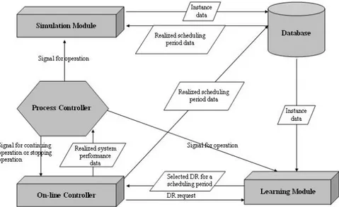
The goal of the proposed system is to select the best dis-patching rule (DR) among Candidate Disdis-patching Rules (CDRs) for a particular scheduling period. The general structure is shown in Figure 1. In this structure, there are five main subroutines, called modules. They operate in harmony to achieve the goal of selecting the best perform-ing dispatchperform-ing rule for each schedulperform-ing period (time inter-val during which a selected DR is used to schedule jobs) throughout the planning horizon. The database provides necessary data for both the learning module and the simu-lation module. It holds the instance data, which is com-posed of a number of attributes and a class value where at-tributes take values of manufacturing conditions and class value corresponds to the DR selected for a specific condi-tion, for the learning algorithm to generate the learning tree. The realized scheduling period data, which represents the actual events that occur in a specific scheduling period such as the processing times, interarrival times and system conditions at the beginning of the scheduling period, is also stored in the database for assessment of DRs via simula-tion. Note that, realized scheduling period data is
com-posed of random number generator seed numbers when we are experimenting with our approach in a computerized environment rather than a real life manufacturing system.
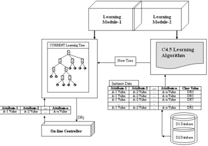
The Simulation module is used to measure the per-formances of the candidate dispatching rules. The simula-tion module is invoked by the process controller module whenever necessary. The simulation module’s outputs (in-stance data) are sent to the database. These results are then used by the learning module to generate the learning tree. The learning module is mainly composed of two parts: learning module-1 (LM1) and learning module-2 (LM2) (see Figure 2). LM1 contains the learning tree that is con-structed by the learning algorithm in LM2. Its responsibil-ity is to select a new DR from the existing learning tree based on the current values of the system state attributes. The on-line controller module provides the current values of these attributes to LM1 and requests a new DR. In re-sponse, LM1 recommends the best DR to the on-line con-troller (see Figure 2). LM2 contains the learning algorithm that is used to generate the learning tree in LM1. As seen in Figures 1 and 2, the algorithm is invoked by the process controller module and the necessary data (instance data) is retrieved from the D2 database. C4.5 algorithms (Quinlan 1993) are used to create the learning tree.
Whenever a scheduling decision is to be made accord-ing to the current schedulaccord-ing strategy (e.g., hybrid ap-proach), the learning tree selects a new dispatching rule and this decision is implemented by the on-line controller module (i.e., it employs the selected DR in actual manufac-turing conditions). It also supplies the realized scheduling period data to the database and monitors the real system for new rule selection symptoms, the triggering events that are defined in the scheduling strategy to answer the question of “when-to-schedule”. The process controller module moni-tors the performance of the learning tree. It takes its inputs
(realized value of average tardiness) from the on-line con-troller module and monitors the performance of the learn-ing tree. When the performance of the current learnlearn-ing tree is found to be insufficient, it requests from the simulation module to provide new training data (instance data) for the learning module and then sends a signal to the learning module to update the current learning tree with this new data set. As a result, new dispatching rules are selected from this updated learning tree and the process continues in this manner.
Figure 2: Learning Module
The scheduling strategy employed in this research is composed of two critical decisions: how-to-schedule and when-to-schedule. The How-to-schedule decision deter-mines the way in which the schedules are revised or up-dated. As discussed in Sabuncuoglu and Goren (2003), there are mainly three issues: scheduling scheme, amount of data used, and type of the response. Our implementation is based on the “on-line” scheduling scheme. Specifically, DRs are selected by the learning tree and the scheduling decisions are made one at a time using these selected rules. In terms of the amount of data, we apply the “full” scheme, and as the type of response, we use the “reschedule” op-tion, since a new DR is selected at any time when the per-formance of the existing DR in use is found to be poor.
“When-to-schedule” determines the responsiveness of the system to various kinds of disruptions. In this research a hybrid approach is employed for “when-to-schedule” de-cisions, in which two different triggering events, called new rule selection symptoms, are defined for determining the time of selecting a new DR. These new rule selection symptoms and their definitions are given in Table 1.
Table 1: New Rule Selection Symptoms
One of the distinguishing features of the proposed scheduling system is its mechanism that continuously up-dates the learning tree. This continuous update is important since the manufacturing system often undergoes various types of changes in time. In this context, the process con-trol charts (X and R charts) act as a regulator of the learn-ing tree. Moreover, the process control charts may also need to be updated due to changes in manufacturing condi-tions. Hence, as the proposed system evolves over time, two important decisions need to be made:
• Is it necessary to update the existing learning tree at current time t?
• Is it necessary to update the existing process con-trol charts at current time t?
These two questions are to be answered every time when a new data point is plotted on the process control charts (X and R charts) and the decisions are made by the rules de-fined in the logical controller sub-module of the process controller module. These rules are defined in Tables 2 and 3 and are adapted from the literature (see, for example, DeVor et. al. 1992).
Table 2: Update Only Learning Tree Rules
Signal Definition Apply to
Extreme
Points Xi or Ri points that fall beyond the control limits of the Xand R charts, respectively.
Xand R charts Zone-A
signal Two out of threeXi points in Zone-A (between 2σ and 3σ) or beyond.
X chart only Zone-B
signal Four out of five Xi points in Zone-B (between σ and 2σ) or beyond.
X chart only
Table 3: Update Both Learning Tree and Process Control Charts Rules
Signal Definition Apply to 8 successive
points 8 or more successive points strictly above or below the centerline Xand R charts 2 successive signals from Rule Set-1
Two successive occurrences of “Update Only Learning Tree Signals”
Xand R charts The learning module of the system generates a learn-ing tree that relies on the manufacturlearn-ing system character-istics. Decisions on selecting dispatching rules are given by the existing learning tree on-line. In such a system, the learning algorithm requires a number of attributes that can provide valuable information about the current manufactur-ing system conditions. These attributes, therefore, play a key role in the performance of the proposed system, since they impact the quality of the tree in the construction phase
as well as in the decision phase (i.e., selection of the right DRs from the learning tree for a scheduling period). Hence, appropriate attributes are defined and used in such a way that they can represent a variety of important manu-facturing system characteristics.
3 EXPERIMENTAL DESIGN AND COMPUTATIONAL RESULTS
3.1 Preliminary Analysis on System Parameters In this section, we present the results of the experiments on the important system parameters, namely the scheduling period (SPL) and monitoring period lengths (MPL). SPL is a time interval during which a selected DR is used to schedule jobs. The rule can be changed before the end of the scheduling period if the performance of the system is found to be worse than a threshold value at the monitoring points. MPL is therefore defined to be the time interval be-tween two successive monitoring points. In the following two sections, we present the results of the experiments on SPL and MPL, respectively. The simulation experiments are carried out under the following assumptions:
• The problem considered is a classical job shop problem with four machines given by Baker (1984).
• There is a set of candidate dispatching rules (CDR) that can be used (i.e., shortest processing time (SPT), modified due date (MDD), modified operation due date (MOD) and operation due date (ODD)).
When explaining the experimental results, we use three performance functions, called Multi-pass Performance (MultiPass), Best Performance (BestPerf) and the Learning Performance (LearnPerf). MultiPass is the average tardiness value achieved by the decisions of a multi-pass scheduling simulator. BestPerf is the minimum average tardiness value that can ever be achieved for a scheduling period, say pe-riod-j, by using any rule given in the candidate rule set. In other words, it is the best average tardiness value that we can achieve in period-j subject to the parameter values of the system, such as the scheduling and monitoring period lengths, the candidate dispatching rules and so on. We can calculate this value for a scheduling period-j only if the re-alization of random events during period-j is already known (i.e., we gather the scheduling period data of period-j). Fi-nally, the learning performance in period-j, LearnPerf, is the realized average tardiness value of the rule selected by the learning tree. Note that, BestPerf gives a lower bound for the other two performance functions.
In the simulation experiments, two levels of utilization (i.e., low and high) and two levels of due date tightness
(i.e., loose and tight) are considered. The two levels of utilization are taken to be 80% and 90%. Due dates are set by using the TWK due date assignment rule. The high and low levels are set in such a way that the percent of tardy (PT) jobs is approximately 10% and 40% under the FCFS rule for the loose and tight due date cases, respectively. 3.1.1 Simulation Results on SPL
As can be seen in Table 4, 11 different levels of scheduling period lengths are tested in the experiments for four due date and utilization level combinations. The simulation re-sults are taken in steady state with 20 replications each with 200000 minutes of a planning horizon. To find Best-Perf, scheduling rules are compared under the same ex-perimental conditions using the common random number (CRN) scheme.
Table 4: Experimental Design of SPL Factors Levels
Scheduling
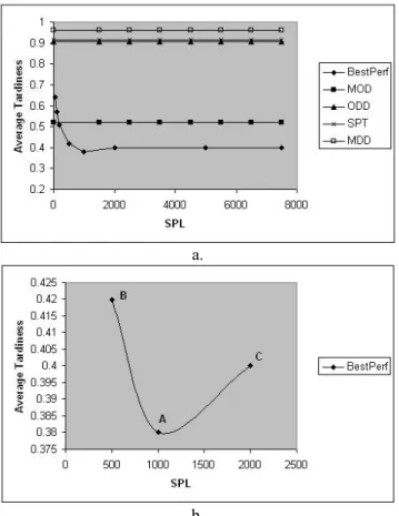
pe-riod length 50, 100, 200, 500, 1000, 2000, 5000, 7500, 10000, 12500 and 15000 The result for the loose due date and 90% utilization case is depicted in Figure 3. Note that, results under 80% utilization case show the same behavior, as well. In this figure, single-pass performances of each dispatching rule are also displayed in addition to BestPerf and single-pass performance of SPT is found significantly worse than the other rules. The single-pass performances of MOD, ODD and MDD are almost equal. Also, BestPerf displays an ex-ponential decay behavior as a function of SPL. It is inter-esting to note that for short scheduling period length selec-tions, BestPerf is found to be significantly worse than the single-pass performances of the three dispatching rules (MOD, ODD and MDD). This is due to the fact that as SPL decreases, even though the selected rules seem to be the best for these short scheduling periods, the system switches to different rules so frequently that the perform-ance of the system in the long run deteriorates. When we increase SPL, BestPerf begins to improve and converges to the single-pass performance of the rules MOD, ODD and MDD. Since the performances of the individual dispatch-ing rules (MDD, ODD and MOD) are very close to each other in the long run for loose due-dates (as also stated by Baker 1984), switching between these rules doesn’t pro-vide any benefit. Therefore, BestPerf converges to a limit (single-pass performance of the rules) showing the behav-ior of an exponential decay function.
For the tight due dates, the experimental results show different behavior to some extent (see Figure 4-a and b). In Figure 4-a, single-pass performances of each dispatching rule are also displayed in addition to BestPerf. It is shown in the figure that the single-pass performances of the four dispatching rules are significantly different than each other
and MOD performs at least twice better than the other rules. In addition, BestPerf displays an exponential decay behavior as we increase SPL, but having a minimum value at some point. For example in Figure 4, BestPerf reaches its minimum value at point A (i.e., SPL equals to 1000 minutes) and then it begins to deteriorate and converges to a limiting value when we further increase the scheduling
Figure 3: BestPerf under 90% Utilization and Loose Due-Dates
a.
b.
Figure 4: 80% Utilization, Tight Due-Dates: (a) Complete Display of the Results. (b) Zoom-In Version around Point A.
period length. We explain this interesting behavior as fol-lows: choosing a shorter scheduling period length results in misdetection of the best dispatching rule for the sake of better long-run performance of the system (i.e., system switches between rules frequently). When we increase the scheduling period length, system begins to select the best rule combination and BestPerf reaches its minimum. But, when we continue to increase the scheduling period length further, performance deteriorates and converges to a higher value than the minimum. This higher value is close to the long-run performance of the most dominant dispatching rule, because the system begins to choose that rule most of the time. Thus, this significant increase in system perform-ance is attributable to the loss of the improvements that can be achieved by switching to different rules during those long scheduling periods.
We also check whether the minimum points achieved in the tight due date case are statistically significant or not. Figure 4-b shows the magnified portion of Figure 4-a around the minimum point. We say that the point A is sta-tistically smaller than the two neighboring points (i.e., points B and C) and this was verified by the paired-t test with 95% confidence.
3.1.2 Simulation Results on MPL
In this section we address the questions of how far the monitoring points should be apart from each other (i.e., the MPL) and what should be the value of the β-parameter, which is a parameter that defines the threshold value on the average tardiness measured at monitoring points. That is, if the average tardiness observed at any monitoring point is larger than β times the expected long run performance of the system ( X ), we select a new DR at that point in time.
A nested experimental design is given in Table 5, in which the factor monitoring period length (MPL) is nested inside the factor scheduling period length (SPL). Note that, MPL of 1000 for SPL being 1000 corresponds to the case of no monitoring at all, since they are equal. 12 levels of the β parameter are used in the experiments. The value of X is taken to be 0.6795 and 1.195 for 80% and 90% utili-zations, respectively. These values are the BestPerf values for 80% and 90% utilizations with respective SPLs (i.e., SPL=1000 for 80%, SPL=7500 for 90% utilization), which we found in the previous section.
As a summary of our results, we found that for both 80% and 90% utilizations, monitoring the system perform-ance at discrete points in time improves our objective func-tion (i.e., average tardiness). Also, experiments show that it is vitally important to select not only the right monitoring period length, but also the right β parameter for that MPL. For example, for the 90% utilization case, a MPL of 2500 with a β value other than 1 results in worse performance measures than no monitoring case (i.e., mean tardiness values greater than 1.195). Moreover, for both 80% and 90% utilizations, system performance improves with small monitoring period lengths. In addition to that, for small monitoring period lengths, small β values work better. For example, for 80% utilization, it is best to choose β=0.2 when MPL=250 whereas β=1 when MPL=500.
3.2 Performance of Learning-Based System
In this section, we test our system with a dynamic learning tree (i.e., all of its modules discussed in Section 2 are acti-vated). In other words, we now continuously monitor the quality of the learning tree by the control charts and update it whenever necessary. Thus, we call this experiment scheduling with a dynamic learning structure.
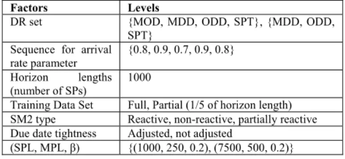
In the simulation experiments, we consider a manufac-turing system in which its internal parameters change in time (i.e., arrival rate, due date tightness levels). The de-tails of the experimental design are given in Table 6. Note that, we use 5 planning horizons, where each horizon con-tains 1000 scheduling periods. At the beginning of each horizon, we change some of the parameters of the manu-facturing system. For example, in Table 6, the factor “pa-rameter sequence for arrival rate” represents the value of the arrival rate of the jobs during each horizon. Specifi-cally, in horizons 1, 2, 3, 4 and 5, jobs arrive exponentially with parameters 0.8, 0.9, 0.7, 0.9 and 0.8, respectively. For the construction of the learning tree, we consider two dif-ferent strategies, which are represented by the factor “Training Data Set” in Table 6. When this factor is at its level Full, the learning tree is constructed based on all the accumulated data points since the beginning of the experi-ment. On the other hand, if its level is set to Partial, the most recent 200 data points (1/5 of a horizon length) are used each time when the learning tree is updated.
We consider three levels for the SM2 type: reactive, non-reactive and partially reactive. When SM2 type is re-active, the multi-pass simulation model is updated immedi-ately when there is any parameter change in the actual manufacturing environment. In other words, if the arrival rate of the jobs changes in real world, this information is made available for the multi-pass simulation model imme-diately. Intuitively, this is impossible in real world imple-mentation, because when any parameter of the manufactur-ing system changes it can be made available to the simulation model of the system after a period of time. This
delay is inevitable since detecting the shift in the parame-ters requires data collection and statistical analysis. For this reason, we also consider the partially reactive level for SM2 type. When the type is partially reactive, the multi-pass simulation model is updated for the arrival rate changes, but with some time delay and an accuracy level. Specifically, arrival rate is updated with a delay of 200 scheduling periods (1/5 of a horizon length) after the actual change in the real world takes place and set to the values in the sequence {0.8, 0.875, 0.725, 0.875, 0.8} for each hori-zon 1 through 5, respectively. The time delay for the up-date represents the passage of time for collecting sufficient data, which is necessary to statistically determine the new arrival rate. As another extreme, we consider SM2 type as non-reactive. In this case the model is not updated for any changes in the manufacturing environment. For example, when the arrival rate changes from 0.8 to 0.9 in the real world, the multi-pass simulation model continues to oper-ate under the initial arrival roper-ate, which is 0.8.
Table 6: Experimental Design for Scheduling with Dy-namic Learning Structure
Factors Levels
DR set {MOD, MDD, ODD, SPT}, {MDD, ODD,
SPT} Sequence for arrival rate parameter
{0.8, 0.9, 0.7, 0.9, 0.8} Horizon lengths
(number of SPs)
1000
Training Data Set Full, Partial (1/5 of horizon length)
SM2 type Reactive, non-reactive, partially reactive
Due date tightness Adjusted, not adjusted
(SPL, MPL, β) {(1000, 250, 0.2), (7500, 500, 0.2)}
Another factor considered in the experiments is due date tightness and it has two levels, adjusted and not ad-justed. For the adjusted case, we set the allowance factor k for setting the due dates such that the percent tardy is al-ways 40% under the FCFS rule. For the not adjusted case, the flow allowance factor is always at the level 5.5 for all arrival rates. Therefore, the first case corresponds to a pol-icy such that the manufacturing firm adjusts its due date setting policy when the arrival rate of the jobs changes and in the second case no action is taken for setting the due dates of the jobs when the utilization of the shop floor changes.
The last factor that we consider in the experiments is the choice of scheduling and monitoring period lengths along with the β value. For the levels of this factor, we simply consider the best combinations that we previously determined for 80% and 90% utilization levels. Therefore, the two levels, (1000, 250, 0.2) and (7500, 500, 0.2), are considered for this factor. At the beginning of each ex-periment, there is a warm up period with a length of 200 scheduling periods to provide necessary initial data to the system to construct the first learning tree and the control charts. System statistics are initialized after the warm up
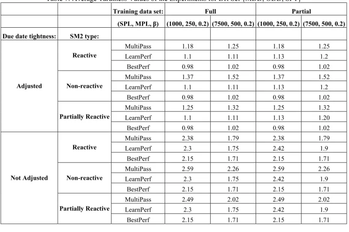
Table 7: Average Tardiness Values of the Experiments for DR Set {MDD, ODD, SPT}
Training data set: Full Partial
(SPL, MPL, β) (1000, 250, 0.2) (7500, 500, 0.2) (1000, 250, 0.2) (7500, 500, 0.2) Due date tightness: SM2 type:
MultiPass 1.18 1.25 1.18 1.25 LearnPerf 1.1 1.11 1.13 1.2 Reactive BestPerf 0.98 1.02 0.98 1.02 MultiPass 1.37 1.52 1.37 1.52 LearnPerf 1.1 1.11 1.13 1.2 Non-reactive BestPerf 0.98 1.02 0.98 1.02 MultiPass 1.25 1.32 1.25 1.32 LearnPerf 1.1 1.11 1.13 1.20 Adjusted Partially Reactive BestPerf 0.98 1.02 0.98 1.02 MultiPass 2.38 1.79 2.38 1.79 LearnPerf 2.3 1.75 2.42 1.9 Reactive BestPerf 2.15 1.71 2.15 1.71 MultiPass 2.59 2.26 2.59 2.26 LearnPerf 2.3 1.75 2.42 1.9 Non-reactive BestPerf 2.15 1.71 2.15 1.71 MultiPass 2.49 2.02 2.49 2.02 LearnPerf 2.3 1.75 2.42 1.9 Not Adjusted Partially Reactive BestPerf 2.15 1.71 2.15 1.71
Table 8: Average Tardiness Values of the Eexperiments for DR Set {MDD, ODD, SPT, MOD}
Training data set: Full Partial
(SPL, MPL, β) (1000, 250, 0.2) (7500, 500, 0.2) (1000, 250, 0.2) (7500, 500, 0.2) Due date tightness: SM2 type:
MultiPass 0.81 0.65 0.81 0.65 LearnPerf 0.81 0.65 0.82 0.68 Reactive BestPerf 0.71 0.6 0.71 0.6 MultiPass 0.96 0.73 0.96 0.73 LearnPerf 0.81 0.65 0.82 0.68 Nonreactive BestPerf 0.71 0.6 0.71 0.6 MultiPass 0.87 0.69 0.87 0.69 LearnPerf 0.81 0.65 0.82 0.68 Adjusted Partially Reactive BestPerf 0.71 0.6 0.71 0.6 MultiPass 1.52 1.2 1.52 1.2 LearnPerf 1.2 1.15 1.61 1.27 Reactive BestPerf 1.15 1.1 1.15 1.1 MultiPass 1.67 1.35 1.67 1.35 LearnPerf 1.2 1.15 1.61 1.27 Nonreactive BestPerf 1.15 1.1 1.15 1.1 MultiPass 1.6 1.26 1.6 1.26 LearnPerf 1.2 1.15 1.61 1.27 Not Adjusted Partially Reactive BestPerf 1.15 1.1 1.15 1.1
period and each experimental condition is run for 5 con-secutive horizons (5000 scheduling periods) as it is given in Table 6. The results of the experiments, MultiPass, LearnPerf and BestPerf, are summarized in Tables 7 and 8. Note that, BestPerf provides the lower bound values for both MultiPass and the LearnPerf.
From these results, our first observation is that our learning-based scheduling system outperforms the simula-tion-based scheduling approach (MultiPass) in 38 ex-perimental conditions out of 48. In these cases, LearnPerf is closer to BestPerf more than MultiPass in a range of 2.34% to 40.87%. In 2 cases, both MultiPass and Learn-Perf are found to be equal. In the remaining 8 cases simu-lation-based scheduling (MultiPass) performs slightly bet-ter than LearnPerf (i.e., between 1.68% and 7.83% better). However, in these cases SM2 type is reactive, which is a difficult condition to achieve in the real world.
When we compare LearnPerf for full and partial training data set cases, we see that using all available data always results in better performance (see Tables 7 and 8). At first glance, this seems to be counter intuitive because when parameters of the manufacturing system change, learning with the most recent data is expected to yield bet-ter performance. However, the results show that our learn-ing algorithm gets benefit from the past data as well as the recent data.
The third observation is related with the selection of SPL, MPL and β values. For the rule set of {MOD, MDD, ODD, SPT}, the combination (7500, 500, 0.2) always gives better results for LearnPerf than the combination (1000, 250, 0.2) (Table 8) regardless of partial or full data sets being used. The reason why the combination (7500, 500, 0.2) yields better results when MOD is in the rule set is that the performance of MOD dominates the perform-ance of other rules when it is used for a long period of time. Thus, the combination (7500, 500, 0.2) yields better results than the combination (1000, 250, 0.2). For the rule set {MDD, ODD, SPT}, the best choice of (SPL, MPL, β) combination depends on the parameter “due date tight-ness”. When the due date tightness factor is at its level not adjusted, the choices of (7500, 500, 0.2) results again in better performance than (1000, 250, 0.2) regardless of the partial or full data sets being used. But, when it is at the adjusted level, (7500, 500, 0.2) and (1000, 250, 0.2) result in better performance for the full and partial training data sets, respectively, (Table 7). These results stress the im-portance of the appropriate selection of SPL, MPL and β values once more.
As stated before, partially reactive SM2 is a more re-alistic case where the simulation model used for the scheduling decisions of multi-pass approach is updated with some time delay and inaccuracy that may exist in de-tecting the parameter changes in the actual manufacturing environment. Therefore, the comparison of the learning-based (LearnPerf) and the simulation-learning-based (MultiPass)
systems for this factor level is of special importance. When the SM2 type is partially reactive, LearnPerf is bet-ter than MultiPass in 14 cases out of 16. That is, Learn-Perf is closer to BestLearn-Perf more than MultiPass in a range of 3.26% to 34.79% in these 14 cases. In the remaining 2 cases, MultiPass is closer to BestPerf more than Learn-Perf only 0.9%, which means they are almost equal. 4 CONCLUSION
In this paper, we present a learning-based scheduling sys-tem for a classical job shop problem with the average tar-diness objective. We perform extensive simulation ex-periments. The results indicate that it is very important to select the appropriate values for SPL, MPL and β. For poorly selected parameters, performance of multi-pass methods can be worse than the single-pass performances of the individual dispatching rules. The results also indi-cate that the proposed system performs better than the simulation-based multi-pass scheduling and the single-pass scheduling. But for very large values of monitoring intervals, the performance of the proposed system deterio-rates to the level of the performance of the multi-pass scheduling system. Hence, at this point we conclude that the monitoring process is really essential for our learning based algorithm. Moreover, when we add a competitive dispatching rule (i.e., MOD) to our rule set, the perform-ance of the proposed system as well as the MultiPass fur-ther improves (gets closer to BestPerf). Hence, deciding the rules in the candidate dispatching rule set is also im-portant for the performance of our learning algorithm. REFERENCES
Cho, H., and Wysk, R.A. 1993. A robust adaptive sched-uler for an intelligent workstation controller. Interna-tional Journal of Production Research 31 (4): 771-789.
DeVor, R. E., Chang, T-h., and Sutherland, J. W. 1992. Statistical Quality Design and Control. New Jersey: Prentice Hall.
Ishii, N., and Talavage, J.J. 1991. A transient-based real-time scheduling algorithm in FMS. International Journal of Production Research 29 (12): 2501-2520. Jeong, K. –C., and Kim, Y.-D. 1998. A real-time
schedul-ing mechanism for a flexile manufacturschedul-ing system: using simulation and dispatching rules. International Journal of Production Research 36: 2609-2626. Kutanoglu, E., and Sabuncuoglu, I. 2001. Experimental
investigation of iterative simulation-based scheduling in a dynamic and stochastic job shop. Journal of Manufacturing Systems 20: 264-279.
Pierreval, H., and Mebarki, N. 1997. Dynamic selection of dispatching rules for manufacturing system
sched-uling. International Journal of Production Research 35: 1575-1591.
Quinlan, J.R. 1993. C4.5 Programs for Machine Learn-ing, California: Morgan Kaufmann.
Sabuncuoglu, I., and Goren, S. 2003. A review of reactive scheduling research: proactive scheduling and new robustness and stability measures. Technical working paper, Department of Industrial Engineering, Bilkent University.
Shaw, M.J., Park, S., and Raman, N. 1992. Intelligent scheduling with machine learning capabilities: the induction of scheduling knowledge. IIE Transactions 24: 156-168.
Suwa, H., and Fujii, S. 2003. Rule acquisition for rolling horizon heuristics in single machine dynamic sched-uling. Proceedings of the 7th World Multiconference
on Systemics, Cybernetics and Informatics 13: 279-284.
Tayanithi, P., Minivannan, S., and Banks, J. 1993. A knowledge-based simulation architecture to analyze interruptions in a flexible manufacturing system. Journal of Manufacturing Systems 11 (3): 195-214. Wu, S.D., and Wysk, R.A. 1988. Multi-pass expert
con-trol system – a concon-trol/scheduling structure for flexi-ble manufacturing cells. Journal of Manufacturing Systems 7 (2): 107-120.
AUTHOR BIOGRAPHIES
GOKHAN METAN is a Ph.D. student in industrial and systems engineering in the Lehigh University. In 2002 he received his M.S. and 2000 B.S. degrees in industrial en-gineering from Bilkent University. His research interests include scheduling, simulation, AI and supply chain man-agement.
IHSAN SABUNCUOGLU is a Professor of Industrial Engineering at Bilkent University. He teaches and con-ducts research in the areas of simulation, scheduling and manufacturing systems. He has over 50 papers in various scientific journals.