Sorting of chiral microswmmers

(1)

SORTING OF CHIRAL MICROSWIMMERS

a thesis

submitted to the department of physics

and the graduate school of engineering and science

of bilkent university

in partial fulfillment of the requirements

for the degree of

master of science

By

Mite Mijalkov

December, 2014

(2)

I certify that I have read this thesis and that in my opinion it is fully adequate, in scope and in quality, as a thesis for the degree of Master of Science.

Assist. Prof. Dr. Giovanni Volpe(Advisor)

Assoc. Prof. Dr. Hande Toﬀoli

Assist. Prof. Dr. Miguel Navascu´es

Approved for the Graduate School of Engineering and Science:

Prof. Dr. Levent Onural Director of the Graduate School

(3)

ABSTRACT

SORTING OF CHIRAL MICROSWIMMERS

Mite Mijalkov M.S. in Physics

Supervisor: Assist. Prof. Dr. Giovanni Volpe December, 2014

Microscopic swimmers, for example chemotactic bacteria and cells, are capable of directed motion by exerting a force on their environment. In some cases, including bacteria and spermatozoa swimming near boundaries, or many asymmetrical ar-tificial microswimmers, the driving force and propulsion direction are misaligned. In those situations a torque acting on the microswimmers arises, resulting in mo-tion with a well-defined chirality which is circular in two dimensions and helicoidal in three dimensions. In this thesis, I demonstrate with numerical simulations in two dimensions, how the chirality of the circular motion can couple to chiral fea-tures present in the microswimmer environment. I show that by employing static chiral pattern of elliptical obstacles in their environment, microswimmers can be separated on the basis of their motion parameters. In particular, levogyre and dextrogyre microswimmers as small as 50nm can be separated and selectively trapped in chiral flowers of ellipses. Patterned microchannels can be used as

fun-nels to rectify the microswimmer motion, as sorters to separate microswimmers

based on their linear and angular velocities, and as sieves to trap microswimmers with specific parameters. I also demonstrate that these results can be extended to helicoidal motion in three dimensions.

(4)

¨

OZET

KIRAL MIKROY ¨

UZ ¨

UC ¨

ULERIN SINIFLANDIRILMASI

Mite Mijalkov

Fizik bölümü, Yüksek Lisans

Tez Y¨oneticisi: Yrd. Do¸c. Dr. Giovanni Volpe Aralık, 2014

Kemotaktik bakteriler ve hücreler gibi yüzen mikroskopik canlılar ¸cevrelerine kuvvet uygulayarak hareket yönlendirebilme yetene˘gine sahiptirler. Bazı durum-larda, örne˘gin, bakteri ve sınıra yakın yüzen sperm, veya bir¸cok asimetrik yapay yüzücülerde, itici kuvvet ve itme yönü yanlı¸s hizalanmı¸stır. Böyle durumlarda; mikroyüzücüler üzerine etki eden, iki boyutta dairesel ve ü¸c boyutta sarmal olan iyi tanımlanmı¸s bir kiralite ile harekete neden olan bir dönme kuvveti ortaya ¸cıkar. Bu tezde, iki boyuttaki nümerik simulasyonlar ile, dairesel hareketin ki-ralitesi ile mikro yüzücülerin ortamında mevcut olan kiral özelliklerin birbiri ile nasıl e¸sle¸sti˘gi gösterilmektedir. Kendi ¸cevrelerindeki eliptik engellerin statik ki-ral desenini kullanarak, mikroyüzücülerin kendi hareket parametreleri temelinde ayrılabildi˘gi gösterilmektedir. Ozellikle, 50nm kadar k¨¨ u¸cük levojir ve dextro-jir mikroyüzüc¨uler elipslerin kiral ¸ci¸ceklerinde ayrılabilir ve se¸cici olarak kapana

kıstırılabilirler. Mikroyüzücülerin hareketini düzeltmek amacıyla, lineer ve a¸cısal hızına dayalı olanları ayırmak i¸cin ayıklayıcı olarak ve belirli parametreler ile olanları yakalamak i¸cin süzge¸c olarak desenli mikrokanallar huni olarak

kul-lanılabilirler. Ayrıca bu sonu¸cların ¨u¸c boyuttaki sarmal harekete uzatılabildi˘gi de g¨osterilmektedir.

(5)

Acknowledgement

I cannot express my gratitude to Dr. Giovanni Volpe enough, for his patience with me when I was starting to learn programming, his guidance, his willingness to listen to my ideas and discuss them and for the opportunity he gave me to work on extremely good projects, helping me develop as a person who enjoys his work. I sincerely believe that there is no-one in the academic circles that could do more for me and I feel honored that I could spend three fruitful years working with him.

A special thanks to Dr. Hande Toﬀoli and Dr. Miguel Navascu´es for their agree-ment to be in this thesis’ comitee and provide insight to make it as good as possible. Also, I would like to express my thanks to Prof. Atilla Er¸celebi for his guidance when I needed the most, upon enrolling in the physics department in Bilkent.

I would like to give my best wishes to all my friends that I met in METU and Bilkent as well as all the members of the Soft Matter group in Bilkent. You were all special to me and I will always cherish the small moments in life that I shared with you, the drinking after a hard homework, drinking in a pub, drinking in the oﬃce, picnics, coﬀee breaks and conference travels. I wish you all the best with your life, and hope you obtain your goals and find true happiness. I hope we could meet in future and create new and better memories.

To my uncle Sterjo, my parents Dimce and Ivanka, it goes without saying that I would not have been here without your continuous support, understanding and motivation. I will do my best to repay for all the incredible things you have done for me, but I honestly believe that one lifespan would not be enough to show my true gratefulness to you.

Finally, Merve, I hold you near and dear to my heart. The day to day support that you gave me during these past 8 months have been unimaginable and I cannot believe I was so lucky to meet such a kind and understanding person. You impress me more and more with every passing day and I hope to see your beautiful face and charming smile for the long years to come.

(6)

List of Figures

2.1 Illustration of binary random walk . . . 5

2.2 Random walk paths of three walkers . . . 6

2.3 MSD as a function of time for 4 diﬀerent walkers . . . 8

2.4 Average distance vs time in ensemble average . . . 9

2.5 Probability transitions and sum rule . . . 11

2.6 White noise simulation . . . 14

2.7 A single realization of white noise and the resulting one and two dimensional motions. . . 15

3.1 Three trajectories of the Brownian motion of granules as recorded by Jean Perrin . . . 18

3.2 Comparison between the inertial and non-inertial regime . . . 28

3.3 Numerical solution of the free diﬀusion equation . . . 29

3.4 Evolution of the probability distribution of an ensemble of 100 Brownian particles in 2D square well . . . 30

(10)

LIST OF FIGURES x

4.2 Examples of artificial systems for self-propulsion at the microscale 33

4.3 Active Brownian motion tunable by light . . . 34

4.4 Active Brownian motion of particles as function of particle radius and velocity. MSD as a function of time for active swimmers . . . 37

4.5 Evolution of the probability distribution of an ensemble of 100 active Brownian particles with propulsion velocity of 1µm/s in 2D square well . . . 38

4.6 Evolution of the probability distribution of an ensemble of 100 active Brownian particles with propulsion velocity of 50µm/s in 2D square well . . . 38

5.1 Chiral motion in homogeneous environment . . . 42

6.1 Illustration of periodic boundary conditions . . . 45

6.2 Original vs unwrapped trajectory in the case of periodic boundary conditions . . . 46

6.3 Sliding boundary conditions inside a circular well . . . 48

6.4 Sliding boundary conditions for a microswimmer encountering el-liptical obstacles in its environment . . . 50

7.1 Chiral microswimmers in a chiral environment . . . 52

7.2 Separation of levogyre and dextrogyre microswimmers . . . 56

7.3 Sorting eﬃciency . . . 57

7.4 Linear velocity based sorting in a microchanne . . . 58

(11)

LIST OF FIGURES xi

(12)

List of Tables

(13)

Chapter 1 Introduction

Most of the events that we frequently encounter are inherently random. Ran-domness takes place in many sciences including game and information theory, and is also used to model stock markets, games of chance, etc. [1]. Due to its widespread use, there have been great interest to model and gain an intuitive un-derstanding of these phenomena. However, solving the corresponding equations is a tough task due to the requirement of complex mathematical understand-ing. Often, processes are simplified by doing some justifiable approximations and solving simpler models that serve as a paradigm to understand more complex behavior.

One of the simplest stochastic processes that can be studied is the Brownian motion [2]. This is the omnipresent and continuous random motion of any micro-scopical particle suspended in a fluid that arises due to the continuous collisions with the surrounding fluid molecules. As such, it has been a model and inspiration for many discoveries, in particular the development of the microscopic theory for the matter structure [3]. Moreover, since the Brownian motion exists in thermal equilibrium as a fluctuation, it can be used as model for systems in the scope of equilibrium statistical mechanics.

In contrary to the Brownian particles, which fluctuate randomly while their av-erage position remains at zero, active Brownian particles, also referred to as microswimmers, are able to take up energy from the environment and use it to

(14)

navigate through the environment [4]. They have a well directed motion, which is disturbed by random fluctuations due to their Brownian nature. Due to this property, active swimmers possess the potential to be used in many applica-tions which would include any kind of pick up and delivery of molecules at the nanoscale, then to localize pollutants in soils or to perform tasks in lab-on-a-chip devices [5, 6, 7, 8]. Additionally, their ability to self-propel means that active swimmers are out of equilibrium, so their behavior could be used to model such systems [4]. All these promising applications led to a great interest to study microswimmers and many artificial swimming methods to solve the problem of self-propulsion have been proposed [9].

However, often microswimmers are designed to be asymmetric and the self-propulsion direction does not align with the driving force [10]. In these cases microswimmers become chiral and they undergo a circular motion in two and he-licoidal motion in three dimensions. Such examples are vast, and they also exist in nature, for example the bacterium E. coli and spermatozoa swim in circles when they are near a boundary [11, 12, 13, 14, 15, 16, 17].

Sorting chiral microswimmers based on their swimming properties is of topmost importance in science and engineering. For example, in order to increase the probability of success of the artificial fertilization, velocity based selection of the spermatozoa might be employed [18]. Separation and sorting of some geneti-cally engineered bacteria can be achieved using the morphological variations in the motion parameters [19]. Moreover, the capability of microswimmers to per-form a specific tasks, such as bioremedication or drug delivery, can be significantly increased just by selecting the swimmers that possess the most appropriate swim-ming properties. Finally, the need to separate the chiral (levogyre and dextro-gyre) molecules is very pronounced because generally only one specific chirality is needed by the pharmaceutical and chemical industry [20]. Molecules can be made active by coupling them with a microscopic chiral propellers, and then remove the propellers after the separation is completed. The extreme importance in the methods presented in this thesis, lies in the fact that due to the small Reynolds number of the environment in which the molecules exist, their separation due to chirality is very diﬃcult to achieve by mechanical means [21].

(15)

chiral swimmers can be sorted and separated due to their chirality, linear and an-gular velocity by placing some static patterns in their environment [22]. I explain how to numerically solve the Langevin equation for the motion in homogeneous environment (chapters 2-5), complex environment (chapter 6) and finally I present my results of how to sort chiral microswimmers (chapter 7). First, in chapter 2, I go over some simple definitions of the random walk before outlining the finite diﬀerence method and show how to numerically simulate the white noise. Using these concepts, I demonstrate how to numerically simulate a Brownian parti-cle (chapter 3), active Brownian motion (chapter 4) and chiral microswimmers (chapter 5). Then, in chapter 6, I show how to treat the most commonly encoun-tered boundary conditions which arise when a microscopic particle encounters any obstacle in its environment. In here, I first outline the procedure of treat-ment of periodic and reflective boundary conditions and then I present the sliding boundary conditions illustrated in the examples of particle in a spherical well and microswimmer encountering an elliptical obstacle. Finally, I introduce my results and show that a racemic mixture of two dimensional chiral microswimmers can be separated by placing the microswimmers inside a chiral flower which traps microswimmers with specific chirality. Moreover, I show that a patterned

mi-crochannel can be used as a funnel which rectify the motion of the swimmers, as

a sorter on the basis of the linear and angular velocities of the microswimmers and as a sieve to trap the microswimmers with certain properties. Moreover, I demonstrate that all the results can be extended to the three dimensional case. All these results are scalable down to smaller microparticles as long as the P´eclet number of the motion is kept constant.

(16)

Chapter 2 Random Walk

Random walks are used to model many phenomena occurring at diﬀerent scales, such as scattering of the light at the nanoscale, the motion of biomolecules and nanodevices at microscale or the financial status of a gambler, stock markets or food foraging. Two properties of the random walk are of utmost importance [23]:

scale invariance, the random walks look the same at all scales, and universality,

random walks have the same properties regardless of their nature. Therefore, I discuss some general properties of the random walk in this chapter as an outline of the physical view of Brownian motion that I introduce in Chapter 3. First, I consider the binary unbiased random walk and derive average quantities and the diffusion equation for this model. Then I introduce the finite difference method and go over the procedure of numerically simulating the effects on white noise, before I end this chapter by describing the generalized version of random walk and show the properties of this stochastic process via numerical simulations.

2.1 Binary unbiased random walk in 1D

Binary random walk in 1D occurs when the walker can choose to go in one of the two available directions, making steps of equal length in the process. If the two choices can occur with same probabilities the walk is said to be unbiased, the

(17)

walk is biased if one event is more likely to occur then the other (i.e. the walker experiences a kind of drift in either dimension).

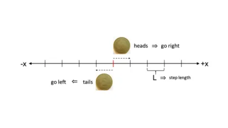
In particular, consider the case in which we have a walker in 1 dimension who makes a decision to go left or right based on the outcome of a simple coin flip. All the steps are of equal length, L, as depicted in figure 2.1.

Figure 2.1: Illustration of binary random walk. The walker makes a decision based on a coin flip: he goes right if the result is heads and left if tails. All the steps are of equal length, L. This is a unbiased random walk since the coin is fair, there is 50% probability to go in either direction.

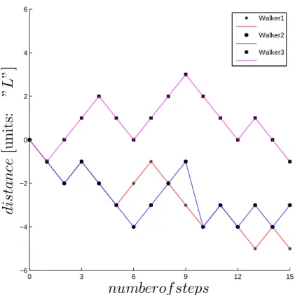
In order to show how the motion looks, I simulate three random walkers that take 15 steps each and show them in figure 2.2. Any individual step is denoted by the black markers, the colors indicate the distinctive paths of the walkers. From figure 2.2, we observe that all the walks are rugged, unlevel, independent and diﬀerent from each other. Subsequently, the individual displacements after

N steps, DN vary from walker to walker. As a result, some variables need to be derived that will answer the questions about how far the walker goes on average in a given time, or how much time does the walker need to get to some certain distance.

(18)

0 3 6 9 12 15 −6 −4 −2 0 2 4 6

numberof steps

d

is

ta

n

ce

[u

n

it

s:

”

L

”

]

Walker1 Walker2 Walker3

Figure 2.2: The path that three walkers take (in units of L) as a function of the number of steps taken in the fair coin toss game. Black markers denote each individual step of the walkers.

2.2 Average quantities

Consider the binary random walker that can make steps with length ±L. Then, if DN is the distance covered in N steps, we can express this distance as a sum of the individual steps,

DN = L1+ L2+ L3+ ... + LN = N ∑

i=1

Li (2.1)

Taking the average and keeping in mind that the average for a single step in an unbiased random walk is 0, we get

DN = L1+ L2+ L3+ ... + LN = L1+ L2+ L3+ ...LN = 0 (2.2) Therefore, the average position of an unbiased random walk is zero. This means that, if we plot the probability distribution of finding the walker at some

(19)

distance, it will be centered at the origin and it will have its tails expanding as the number of steps increases.

The quantity that gives the information of how much the walker traveled from the initial point after some certain number of steps N is the square of the distance,

D_N2. To find the expectation value of D2_N, we simply square 2.1. Then,

D2 N = (L1+ L2+ L3+ ... + LN)2 = N ∑ i=1 Li2+ N ∑ i=1 N ∑ j̸=i LiLj (2.3)

Now, calculating both terms in the sum one by one, (Li)2 = LiLi = 1 2[(+L)(+L) + (−L)(−L)] = L 2 _(2.4) LiLj = 1 4[(+L)(+L) + (−L)(−L) + (+L)(−L) + (−L)(+L)] = 0 (2.5) Therefore, D2_N, or the mean square displacement from the starting point, we have [23] ⟨D2 N⟩ = N ∑ i=1 L2 = N L2 (2.6)

So, the mean-square displacement of an unbiased walker is proportional

to the number of steps.

One more measure for a random walk, is the information of how much time it takes to the walker to reach a certain distance. Consider that it takes the walker

t0 seconds to make a single step with some velocity v. Then, during the total

time t, the walker will make N = _tt

0 steps with length L = vt0. Then,

⟨D2

N⟩ = NL

2 ₌ t

t0

(vt0)2 = (vt0)vt = (vL)t (2.7)

Therefore, we conclude that the the mean-square displacement of an

unbi-ased walker is proportional to the time.

Figure 2.3 shows the calculated MSD (mean-squared displacement) for 4 diﬀerent step lengths. It can be seen that the MSD is proportional to the number of steps (also proportional to time, since t = N t0) and it also illustrates the fact that

(20)

0 25 50 75 100 0 0.5 1 1.5 2 2.5 3x 10 7

M

S

D

[L

2

s

− 1

]

no.of steps

step length = 3L step length = 7L step length = 10L step length = 13L

Figure 2.3: MSD as a function of time (or number of steps) for 4 diﬀerent walkers. Each walker takes a step with diﬀerent length and they all walk for 100L steps. It shows that MSD depends greatly on the step size and is directly proportional to the time elapsed in motion.

An important point to note here is that the above properties were obtained by taking time averages, i.e. considering a particular trajectory of a single random walker and averaging it over time. However, the random walk represents an

ergodic system, so if we take ensemble averages, i.e. considering a lot of random

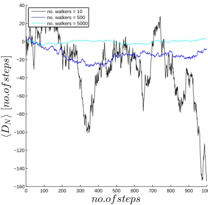
walkers and averaging their trajectories at the same time, the obtained results will coincide. To illustrate this point, I calculate the average distance over a lot of random walkers and plot its evolution over time in figure 2.4. This figure illustrates the point that if we take larger and larger ensembles of walkers, the average of their trajectory approaches the equilibrium position.

(21)

0 100 200 300 400 500 600 700 800 900 1000 −160 −140 −120 −100 −80 −60 −40 −20 0 20 40

hD

N

i

[n

o

.o

f

s

te

p

s]

no.of steps

no. walkers = 10 no. walkers = 500 no. walkers = 5000

Figure 2.4: Average distance as a function of time when averaged over 10 (the black line), 500 (the blue line) and 5000 (cyan line). The average distance goes to zero as we average over larger ensembles. Due to the fact that the system is ergodic, averaging over ensembles gives the same results as averaged over time as shown in section 2.2.

2.3 Continuum limit

In the previous sections, I described the random walk and showed some of its properties by using individual trajectories and analyzing their behavior. However, another way to look at the random walk, is to describe the behavior in terms of the probability to find the walker at a certain position and analyzing how this probability evolves over time. Before outlining these properties, I first explain the finite diﬀerence method, that is used thoroughly throughout this thesis to simulate various motions.

(22)

2.3.1 Numerical

simulations:

The

Finite

diﬀerence

method

In this method [24, 25], I use finite diﬀerences in order to approximate the deriva-tives in the stochastic equations. In particular, the following expression approxi-mates the first derivative in backward diﬀerence:

f′(x)≈ f (x)− f(x − ∆x)

∆x (2.8)

In order to approximate the second derivative, again in the backward direction, I use the following:

f”(x)≈ f (x)− 2f(x − ∆x) + f(x − 2∆x)

(∆x)2 (2.9)

2.3.2 The Diﬀusion equation

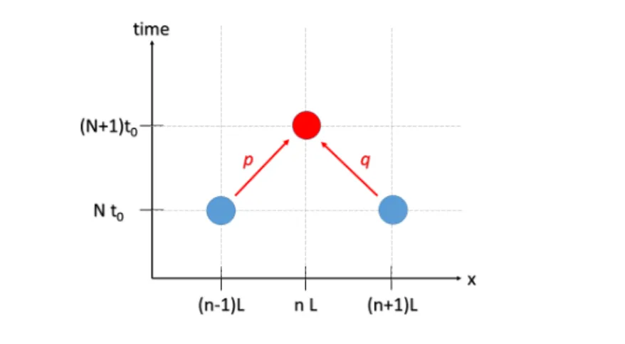
Consider a random walker that has a probability p to take a step to the right and probability q to take a step to the left. Let PN(n) be the probability to find the walker at position DN = nL after time t = N t0. This random walk has the

properties that the probabilities to go from one position to another, in this case

p and q are constant in time, do not depend on the history of the system and

obey the sum rule. Due to these properties, the following equation follows for the probabilities:

PN +1(n) = pPN(n− 1) + qPN(n + 1) (2.10)

This equation represents the following: If the particle is at position DN +1(n) = nL at time t = (N + 1)t0, then there is p chance that the particle came with a step

to the right from DN(n− 1) = (n − 1)L at time t = (N)t0 and there is q chance

that the particle came with a step to the left from DN(n + 1) = (n + 1)L at time

t = (N )t0 as outlined in figure 2.5

From this point on, I will continue the derivation for the specialized case of unbiased random walk. i.e. p = q = 1₂. However, the diﬀusion equation that will be obtained at the end holds in general as I show in the following chapters of this

(23)

Figure 2.5: Probability transitions and sum rule. The particle can reach its final state (the red circle) from two possible positions that could occur 1 time step earlier (the blue circles). Therefore the total probability for the particle to be found at the red circle’s position is the sum of the probabilities for the particle to be found at the positions of the left (right) blue circle and make a next step to the right (left).

thesis.

In this special case, the equation 2.10 becomes:

PN +1(n) = 1

2PN(n− 1) + 1

2PN(n + 1) (2.11)

Subtracting PN(n) from both sides yields

PN +1(n)− PN(n) = 1

2(PN(n− 1) + PN(n + 1)− 2PN(n)) (2.12) Consider the expression on the left. It gives the diﬀerence between the probabili-ties obtained at two consecutive times. In accordance to the discussion in section 2.3.1, in the limit when N is large (thus t0 ≪ t) this finite diﬀerence represents

the time derivative of the probability distribution. In order to preserve the units, this has to be multiplied by t0.

By going through the same arguments, the finite diﬀerence on the right represents the second derivative of the probability with respect to position, multiplied by

L2_{. Therefore, equation 2.12 turns into,}

t0 ∂P ∂t = 1 2L 2∂ 2_P ∂x2 (2.13)

Finally, this can be rewritten as,

∂P ∂t = D

∂2_P

(24)

where D is the coeﬃcient of diﬀusion given by D = _2tL2

0. Equation 2.14 is known

as free diﬀusion equation that describes the evolution of the probability

for a random walk. For the case when all the particles start at the origin, the

diﬀusion equation has the following solution,

P (x, t) = √ 1

4π∆te −x2

4∆t; (2.15)

where, x = nL and t = N t0

2.4 Random walk as a stochastic process

Until now, in the 1D random walk that I considered, the walker was able to move left or right on a lattice with equal steps of length L. However, in the most general case, the lengths do not need to be same, in fact they can also be chosen to be random. Therefore, the random walk can be described as a stochastic process by the following simple free diﬀusion equation:

∂x

∂t = ξ(t) (2.16)

ξ(t) is called white noise and it is the term that gives the randomness of the

system. Intuitively, this equation represents the straightforward interpretation of a random walk: the increments the walker takes over time are variables that are chosen at random.

In the following, I will first discuss the properties of the white noise and how to simulate it numerically, then I illustrate some of the properties discussed above by numerical simulations of random walk.

2.4.1 White noise properties and simulation

The white noise carries the following properties: [25]

(25)

2. Two instances of the noise that occur at diﬀerent times are independent of each other

3. ⟨ξ(t)2_{⟩ = 1 for all ( t)}

In order to represent this noise within the finite diﬀerence approach, we need a discrete sequence of random numbers that will have the same properties as white

noise, thus imitating its behavior. As argued in [25], due to property 1 and 2

described above, we require a sequence of uncorrelated random numbers that has a mean zero. As authors also point out, if we further require the condition

⟨(ξ(t)∆t)2_⟩

∆t = 1, due to the fact that the power of ξ(t) is unitary, the random number

sequence should have a variance of _∆t1 . Since the random number sequences generated by most programming languages are Gaussian sequences with zero mean and unit variance, we need to scale down the random number sequence by dividing it by √∆t to obtain the correct variance.

Finally, the white noise term ξ(t) is described in the finite diﬀerence approach as the

ξ(t) = √ξi

∆t (2.17)

where ξi is a sequence of random numbers generated by any programming lan-guage. One particular instance of the white noise is shown in figure 2.6

2.4.2 Numerical simulation of general random walk

In view of the discussion above about the treatment of white noise and the deriva-tive within the finite diﬀerence approach in section 2.3.1, equation 2.16 takes the following form: xi+1− xi+1 ∆t = ξ(t) √ ∆t ⇒ xi+1= xi+ √ (∆t)ξi (2.18)

If we would like to consider random walk in 2 or 3 dimensions, it is suﬃcient to notice that the motion along diﬀerent Cartesian coordinates can be simulated independently. Therefore, the set of equations that simulate 2D random walk are

xi+1= xi+ √

(26)

0 250 500 750 1000

m

a

g

n

it

u

d

e

[a

.u

.]

random no. sequence

Figure 2.6: One particular occurrence of white noise simulated by using a se-quence of 1000 random numbers generated by MATLAB scripting language with a time step of ∆t = 0.5

yi+1 = yi+ √

(∆t)ξyi (2.20)

where ξxi and ξyi are mutually independent random noises.

In order to illustrate the previous discussions, I plot a single instance of the random walk in figure 2.7. Parts (a-c) show the particular realizations of the white noise needed to simulate the random walks in (d-f) in one and (h-j) in two dimensions respectively. All trajectories are 10s long and we observe that as the time step is decreased, the random walk becomes more jagged and we need a larger magnitude of the white noise to simulate the motion. However, due to the fact that all random walks look similar to each other at all scales, this simulation does not depend on the time step chosen and there is no optimal time step for this free diﬀusion equation. What is more, random walks in x and y direction in figure 2.7 (d-f) are obtained by separating the two components of the two dimensional motion shown in (h-j) thus demonstrating that the Cartesian components of two and three dimensional random walks behave independently of each other.

(27)

−10 −5 0 5 10 ξi WN in x WN in y 0 5 10 15 20 −4 −2 0 2 4 6 8 x (t ) , y (t ) time RW in x RW in y −5 0 5 −2 0 2 4 6 8 y (t ) x(t) −10 −5 0 5 10 0 5 10 15 20 −4 −2 0 2 4 6 8 time −6 −4 −2 0 2 −2 0 2 4 6 8 x(t) −10 −5 0 5 10 0 5 10 15 20 −4 −2 0 2 4 6 8 time −4 −2 0 2 4 6 −2 0 2 4 6 8 x(t)

(a)

(b)

(c)

(d)

(e)

(f)

(h)

(i)

(j)

∆t = 1 ∆t = 1 ∆t = 1 ∆t = 0.5 ∆t = 0.5 ∆t = 0.5 ∆t = 0.1 ∆t = 0.1 ∆t = 0.1

Figure 2.7: Simulation of one particular realization of random walk with tra-jectories that are 10s long.As the time step decreases the tratra-jectories look more ragged and white noise of larger magnitude is needed to replicate the motion. (a-c) The instances of the white noise needed to simulate the one dimensional (d-f) and two dimensional (h-j) random walk. The trajectories in (h-j) are con-structed by concatenating both one dimensional trajectories in (d-f) showing that in two dimensional random walk, each of the x and y components performs an independent random walk itself.

(28)

Chapter 3 Brownian Motion

Brownian motion is the everlasting zigzag motion of the entities present at the microscale. From its earliest observation in the early 19th _{century, Brownian}

mo-tion has constantly gained much attenmo-tion from scientists all around the world. The complete formulation of its theory was done in the early 20th _{century and}

from that point on, the many studies of this motion resulted in its widespread application. In this chapter, after going through a very brief historical overview, I present an outline of the theory of Brownian motion as developed by Einstein and Langevin. Finally, I explain how to simulate this motion by using the finite diﬀerence method explained in Chapter 2 and demonstrate some of its properties by numerical simulations. As the generally accepted picture of the Brownian mo-tion is the one of a microscopic colloidal particle performing random momo-tion due to the collisions with the surrounding molecules, there will be many similarities between the concepts presented here and the ones presented in Chapter 2.

3.1 History

Robert Brown was a botanist who first observed the irregular motion of the pollen grains when suspended in water. He thought that this motion was due to the fact that the grains were living and he was looking for the ”vital forces”,

(29)

interpreting his observations as a motion of small living creatures. However, after experimenting with a vast range of plants of diﬀerent age as well as inorganic grains, he concluded that the motion was an intrinsic property of the microscopic entities, not connected with biology, rather with physics itself.

Afterwards, around 1880s, a series of experiments done by Leon Gouy showed that the motion cannot be due to external forces, but is a property of the fluid itself. Then, the Brownian motion gained its theoretical interpretations. It all started with the works of Einstein who derived the expressions for the diffusion constant and mean-squared displacement of a suspended particle. Then, Smoluchowski obtained the same results as Einstein but with a different numerical coefficient and finally, Langevin showed a mistake in Smoluchowski’s assumptions and provided a much simpler derivation of the diffusion coefficient. These results provided a good framework for Jean Perrin to make his careful, precise and systematic experiments that showed the first quantitative observations of the Brownian motion. [26]

3.2 Basic properties

Figure 3.1 below shows three trajectories of Brownian particles recorded by Per-rin. He was tracking small granules (the radius of the granules being 0.52µm) suspended in water by recording the positions of the granules every 30 seconds and then connecting the positions (black dots in the figure) by straight line seg-ments in what is one of the earliest experimental systematic study of the Brownian motion.

All careful work on Brownian motion led to the conclusion that the following main properties hold:

• The motion consists of straight translations and rotations at random angles.

It is extremely irregular and the trajectory does not have a tangent (the velocity of the motion is not well defined).

(30)

Figure 3.1: Three independent trajectories of the Brownian motion of granules with radius 0.52µm as recorded in 30s intervals by Jean Perrin in one of the earliest systematic experimental works to measure the properties of Brownian motion. Adapted from [27]

.

not aﬀect each other and move independently.

• The motion becomes more vigorous as: the particles get smaller, the fluid

gets less viscous and the temperature increases.

• The composition of the particles has no eﬀect on the motion. • The motion is omnipresent at microscale and does not ever stop.

3.3 Einstein’s theory of Brownian motion

Einstein’s development of the theory consists of two main results. The first one connects the diffusion coefficient to the other physical parameters describing the system, while the second result is the derivation of the free diffusion equation which describes the evolution of the probability distribution of a particle. In the following, I will go over the main points of both derivations, using the same

(31)

notation as used in [3]. All the following arguments are derived by using 1D systems, however the extension to 2D and 3D is straightforward.

3.3.1 Diﬀusion constant

According to Einstein’s view, the suspended colloids in a solution perform random walk due to the random impulses these colloids experience because of numerous collisions with the solvent’s molecules. He also asserts that the suspended par-ticles and the surrounding molecules are indistinguishable with respect to the osmotic pressure, expressed as

p = kBT ν (3.1) where ν represents the number of suspended particles in unit volume. The ar-gument runs along the following lines: Let ν amount of particles be suspended in a liquid in equilibrium. Furthermore, assume that they are acted upon some external force K (the origin of this external force need not be specified) and the system is in equilibrium. In this configuration, the external force is balanced by the force due to the osmotic pressure of the suspension. Therefore,

Kν− ∂p

∂x = 0 (3.2)

From equation 3.1, substituting for the pressure and taking into account that only the quantity ν depends on x,

Kν− kBT

∂ν

∂x = 0 (3.3)

The next step is to consider unit area and calculate how many particles pass through that area in unit time due to the motion of the suspended colloids. This motion can be analyzed as an interplay between two processes that occur in opposite directions: the external force K pushing a single particle and imparting a certain velocity to it opposed by a process of diﬀusion produced by thermal molecular movement.

According to Stokes’ law, if the suspended particles are spheres with radii R in a liquid with viscosity η, upon the influence of the force K each particle gains

(32)

a velocity _6πηRK . Therefore, a total of _6πηRνK particles pass the unit area in unit time. In addition, if we denote the coeﬃcient of diﬀusion by D, then a total of

−D∂ν

∂x particles pass through the same are in unit time. Since the particles are at equilibrium,

νK

6πηR + (−D

∂ν

∂x) = 0 (3.4)

Substituting the value for νK from equation 3.3, equation 3.4 becomes ( kBT

6πηR − D)

∂ν

∂x = 0 (3.5)

Then, the diﬀusion constant is obtained as

D = kBT

6πηR (3.6)

which is the first main result derived originally by Einstein in ref. [3].

3.3.2 Probability distribution

Let us assume that the probability of a particle to be at a position x at time t is given by f (x, t). Then, in the subsequent very short time interval τ , suppose the particle takes a very short step of magnitude ∆. There will be a certain probability law that will hold for ∆, ϕ(∆), representing the probability of the jump with specific length ∆ happening. In terms of ϕ, the total probability is

expressed as, _∫

+∞

−∞

ϕ(∆) = 1 (3.7)

In addition, there will be equal probabilities of going left and right, so ϕ(∆) =

ϕ(−∆) will hold.

Then, the aim is to calculate the number of particles that are located between x and x + dx at time t + τ .

f (x, t + τ )dx =

∫

f (x + ∆)ϕ(∆)d∆ (3.8) Since we consider a very small increment of time τ , we can expand the left hand side to first order,

f (x, t + τ ) = f (x, t) + τ∂f (x, t)

(33)

Similarly, because ∆ is also very small, f (x + ∆, t) = f (x, t) + ∆∂f (x, t) ∂x + ∆2 2! ∂2_{f (x, t)} ∂x2 . . . (3.10)

Bringing this expression under the integral (bearing in mind that f (x, t) does not depend on ∆) and combining the two equations,

f (x, t) + τ∂f (x, t) ∂t = (3.11) f (x, t) ∫ ϕ(∆)d∆ + ∂f (x, t) ∂x ∫ ∆ϕ(∆)d∆ +∂ 2_{f (x, t)} ∂x2 ∫ ∆2 2 ϕ(∆)d∆ . . .

Consider the right hand side: The second, fourth, sixth and all consecutive terms will vanish because of the property that the probability law is an even function. The fifth, seventh and next terms are ignored because of the high powers of ∆, and the integral in the first term is equal to 1. Therefore, identifying the diffusion coefficient as the second moment of the probability law, in other words the variance, D = 1 τ ∫ +∞ −∞ ∆2 2 ϕ(∆)d∆ (3.12) the diffusion equation is obtained,

∂f (x, t) ∂t = D

∂2_{f (x, t)}

∂x2 (3.13)

In the discussion until now, all of the particles’ positions were taken relative to a single coordinate system. However, due to the randomness and independence of the particle trajectories from each other, Einstein argues that it is possible to consider every particle as an independent system whose origin corresponds to the center of the particle initially, at t = 0. In that case, the solution of the diﬀusion equation is expressed as,

f (x, t) = √n

4πD

e−4Dtx2

√

t (3.14)

where n is the total number of particles. From here, we are able to read oﬀ the mean square displacement of the motion as

(34)

3.3.3 Fokker-Planck equation

The previously derived free diﬀusion equation is the equation of ”motion” of the probability distribution of the Brownian motion. The generalization of this equation in the case in which there is also an external force acting on the particle is known as Fokker-Planck equation. This equation can be derived by introducing the diﬀusion current, which satisfies the continuity relation and is expressed as,

Jdif f(x, t) =−D

∂f (x, t)

∂x (3.16)

If there is any external force applied to the particle,F (x, t), the velocity of the particle can be written as v(x, t) = F (x,t)_γ , γ being the friction coeﬃcient of the suspended particle in the liquid. The total current of particles can be written as

J (x, t) = Jdif f(x, t) + Jext(x, t) =−D

∂f (x, t)

∂x + v(x, t)f (x, t) (3.17)

Then, by taking one position derivative of the right side and invoking the conti-nuity relation, the Fokker-Planck equation is obtained:

∂f (x, t) ∂t = ∂F (x, t)p(x, t) ∂x − D ∂2_{f (x, t)} ∂x2 (3.18)

3.4 Langevin description of Brownian motion

As seen from the previous section, there are 2 ways to describe the Brownian motion: in terms of probability density distribution of an ensemble of particles that evolves over time (its evolution is given by Fokker-Plank equation) or as a stochastic trajectory of a single particle. Both approaches are intrinsically connected, since the probability can be obtained by averaging over many tra-jectories, or on the other hand, the statistical properties of the random forces depend strongly on the probability density distributions. Einstein’s derivation of the diﬀusion equation and its connection to the diﬀusion constant are connected with the 1st_{approach. The Langevin approach is concerned with the derivation of}

an equation whose solution describes a stochastic trajectory of a single Brownian swimmer. In this section I outline the derivation of the Langevin equation and present a way to solve it numerically, via the method of finite diﬀerences.

(35)

3.4.1 Langevin equation

Consider a spherical particle with radius R and velocity v suspended in a liquid with a viscosity η. The motion of the particle can be described by the Newton’s equation:

m∂

2_x

∂t2 = Ftotal(t) (3.19)

The force on the right side represents the total force due to all external interac-tions that the particle feels at time t. Therefore, by virtue of knowing this force as a function of time exactly, the motion of the particle would be completely deterministic. However, owing to the fact that the force is due to collisions with a large number of molecules present in the liquid, a closed from of this force is un-known. Instead, the force is generally broken down into components that model and represent the eﬀects the particle feels. First, as the particle moves through the liquid, there is a frictional force opposing its motion. This force is given by

−γv, where γ is the friction coeﬃcient given by Stokes’ law, γ = 6πηR. So, the

equation now takes the form,

m∂

2_x

∂t2 =−γv(t) (3.20)

The solution to this equation gives an exponentially decaying velocity. However, the actual velocity of the particle cannot remain at zero, so it follows that the friction force is not the only contribution. Rather, another term in the shape of random or fluctuating force is added to model the random collisions with the molecules of the solvent and the equation attains the following form, [28]

m¨x =−γ ˙x +√2kBT γξ(t) (3.21) where ξ(t) again represents a white noise.

This equation represents the Langevin equation to describe the Brownian motion. Note that, both the fluctuation and friction term in the equation originate from the interactions of the Brownian particle with its environment, as such they are closely connected by the Einstein relation for diﬀusion D = kBT

(36)

3.4.2 Numerical Solution

The finite diﬀerence method can be readily applied to solve the Langevin equation numerically. By using the definitions of the derivatives explained in section 2.3.1 and treating the white noise as explained in section 2.4.1, the Langevin equation takes the following discretized form:

m(xi− 2xi−1+ xi−2 (∆t)2 ) =−γ( xi− xi−1 ∆t ) + √ 2kBT γ 1 √ ∆tξi (3.22) Solving this algebraically to obtain the solution for xi, one obtains [25]

xi = 2 + ∆t(_mγ) 1 + ∆t(_mγ)xi−1− 1 1 + ∆t(_mγ)xi−2+ √ 2kBT γ m[1 + ∆t(_mγ)](∆t) 3 2ξ_i (3.23)

This way of writing this equation places emphasis on the ratio _mγ. It has units of _mN s2_kg = s−1. Therefore, the time τ =

m

γ is the characteristic time scale of the equation (momentum relaxation time). It means that one needs to be particularly careful when choosing the time step of discrete simulation ∆t. It has to be small with respect to the total observation time, nevertheless it has to be chosen suﬃciently larger than τ , so that two succeeding updates of the position can be considered independent of each other. This is in contrast to the random walk discussed in chapter 2, due to the fact that there is not a particular time scale of the random walker considered in that chapter.

3.4.3 Inertial vs Non-inertial solution

Reynold’s number is defined as the ratio between inertial and viscous forces and its value is an indication of how important the inertial forces are in the medium. The value can be approximated as Rvρ_η , where ρ, η are fluid density and viscosity respectively and R is the radius of the particle moving with velocity v. For the systems that I consider throughout this work, the Reynolds number is very low [29]. Therefore, for these kinds of swimmers the inertia plays a negligible role, friction forces are overwhelmingly dominant. In addition, since in typical experiments the time scale is much larger than the τ defined above and the instantaneous velocity and the ballistic regime are not probed, [25] the inertia

(37)

term can be dropped. Therefore, a good approximation to equation 3.21 is the following version of Langevin equation

˙x =√2Dξ(t) (3.24)

which has a simpler numerical solution,

xi = xi−1+

√

2D∆tξi (3.25)

An extensive discussion of the validity of the non-inertial approximation vs the inertial solution is done in [25] and their conclusions are summarized in figure 3.2. In figures 3.2(a) and 3.2(b) the authors simulate 1D Brownian motion solving both inertial, eq. 3.22 and non-inertial, eq. 3.25 solutions and plot them as functions of time. In figure 3.2(a) the time steps used in the simulations are much smaller than the characteristic time of the motion and therefore we can observe a big diﬀerence in both trajectories. However, when the time steps are large enough, as in figure 3.2(b), both trajectories look the same. In these cases, the microscopic details are not observable, therefore the eﬀect of inertia is not noticeable and both trajectories look jagged.

In figure 3.2(c) plots of the velocity auto-correlation function are presented, which give information on how the velocity of the particle at time t′ influences the velocity of the particle at some later time t + t′ and is calculated as

Cv(t) = v(t′)v(t + t′) (3.26) We can observe that while the correlation function of the velocity decays to zero with some time scale in the case of the inertial solution, it goes immediately down to zero when we apply the non-inertial solution demonstrating that it does not have a characteristic time scale in this case. Finally, the authors plot the mean square displacement for both cases. Theoretically, it is expected for ballistic motion to have an MSD proportional to t2 and for diﬀusive motion MSD is proportional to t. The plot in figure 3.2(d) demonstrates that both solutions have the same MSD for suﬃciently long times, therefore making them equivalent in this limit.

Due to the discussions above, in the following chapters I will always set m ≈ 0 and solve the non-inertial version of the Langevin equation.

(38)

3.5 Numerical solution of the free diﬀusion

equation

The free diﬀusion equation, 3.13, can be solved numerically by using the method of finite diﬀerences. Instead of solving for f (x, t), I solve for the discrete series

f (xn, tn) therefore creating a grid that discretizes the position and time indepen-dently. In this solution, the index referring to position is denoted with n and the one denoting the time with m.

Approximate the first time derivative in the forward direction:

∂f (x, t)

∂t |xn,tm ≈

fn,m+1− fn,m

∆t (3.27)

To approximate the second derivative of the position, I use the backward deriva-tive:

∂f (x, t)2

∂2_x |xn,tm ≈

fn,m− 2fn−1,m+ fn−2,m

(∆x)2 (3.28)

After rearranging the terms, I obtain for the probability distribution

fn,m+1 = fn,m+

D× ∆t

(∆x)2 (fn,m+ 2fn−1,m+ fn−2,m) (3.29)

The unit for the diﬀusion constant is m2_s−1_{. In the figure 3.3 I plot the probability}

distribution at different times and use D = 0.5m2_s−1 _{for the diffusion coefficient.}

Note that for the Brownian motion of the molecules, the translational diﬀusion coeﬃcient is of the order ≈ 1 µ2s−1. A comparison between equations 3.25 and 2.18 we see that the value used in this calculation corresponds to macroscopic random walk. In the figure we observe that starting the particles from very sharp Gaussian distribution centered at the origin will result to the flattening of the probability distribution for longer times and asymptotically it becomes uniform (over the region in position that is simulated in the grid. In this case it is the region between x =−0.5 and x = 0.5 m ). Therefore, a Brownian particle moving for an infinite amount of time, goes over every point in space.

(39)

3.6 Brownian motion in 2D square well

In order to further illustrate this probability distribution behavior, I confine a Brownian particle in a two dimensional square well with reflective boundary con-ditions. The method for treating the boundary conditions is explained in sec-tion 6.2. In figure 3.4 we see the time evolusec-tion of the probability distribusec-tion of an ensemble of 100 particles randomly distributed around the origin at t = 0s. We see that while in the beginning most of the particles are stacked near the origin, after 1000000 seconds the probability to find a particle inside any position in the well is uniform. Although these results were calculated using ensembles of 100 particles, due to the ergodicity of the system, the same results could be obtained by calculating the probability due to a single very long trajectory.

(40)

Figure 3.2: Comparison between the inertial and non-inertial regime. The iner-tial and non-ineriner-tial solutions are plotted for small times in (a) which leads to diﬀerence in their behavior. The diﬀerence vanishes in the limit of larger time steps, as illustrated in (b). (c) Plot of velocity auto-correlation function in both cases. The fact that the values of this function drop to zero immediately show that velocity has no characteristic time scales. (d) Plot of the MSD in both cases which shows agreement between the two when long time steps are used. Reproduced from [25].

(41)

−0.50 −0.4 −0.3 −0.2 −0.1 0 0.1 0.2 0.3 0.4 0.5 0.01 0.02 0.03 0.04 0.05 0.06 0.07 0.08 x [m] P (x ,t ) t = 0 t = 2.5 ms t = 50 ms t = 5 s

Figure 3.3: Probability distribution as a function of position in the range [-0.5m,0.5m] for diﬀerent times. The initial distribution of the particles is a sharply peaked Gaussian centered at the origin. As the time passes, the probability distribution becomes flatter, asymptotically becoming uniform.

(42)

−2 0 2 x 10−6 −2 0 2 x 10−6 y[m] x[m] P (x , t) −2 0 2 x 10−6 −2 0 2 x 10−6 y[m] x[m] P (x , t) −2 0 2 x 10−6 −2 0 2 x 10−6 y[m] x[m] P (x , t) −2 0 2 x 10−6 −2 0 2 x 10−6 y[m] x[m] P (x , t) t= 1s t= 10s t= 100s t= 106 s

(a)

(b)

(c)

(d)

Figure 3.4: Evolution of probability distribution averaged over 100 particles in time in square well with side length 4µm. Initially, the particle position is ran-domized near the origin. As the time passes, the probability distribution spreads out, becoming uniform after 1000000s. The radius of all particles is 1 µm.

(43)

Chapter 4 Active swimmers

Active swimmers, or microswimmers, are able to convert the energy they pick up from the environment into kinetic energy, resulting in a directed motion. The range of agents that can be considered active is vast, from insects and birds on the macroscale, to flagellated bacteria or sperm cells in the microscale. Due to their potential for many applications, many artificial microswimmers were devised (for example, Janus particles) which are able to propel themselves by various mechanisms. Another reason to study these microswimmers is the fact that they can serve as a model system for out of equilibrium phenomena and thus, drawing a comparison between the systems outlined in this and previous chapter can give a great insight of these phenomena [4]. In here, I first go over some examples of the active motion, starting from the flagellated bacteria to the artificially engineered Janus particles, then I describe the model I use to simulate the active motion before finally I present the numerical solution and illustrate some properties of the motion by simulations.

4.1 Examples of Active motion

There are two main examples of active motion at the microscale: the run-and-tumble motion which is a property of flagellated bacteria and active Brownian

(44)

motion exhibited by the artificially designed microswimmers. In this section I briefly go over the diﬀerent mechanisms of motion citing some examples of both.

4.1.1 Run-and-tumble of the bacteria

A particular trajectory taken by H. Berg [19] while studying the movement E.

coli in gradients is shown in figure 4.1(a).

Figure 4.1: (a) An example of the run-and-tumble motion of Escherichia coli. The dots denote time steps of 0.1 second. Adapted from [19] (b) An illustration of the behavior of the flagella of E.coli. During a run, they rotate together in counter-clockwise direction and propel the bacteriaum. Once in a while, the flagella change their direction of rotation and they start working out of synch, therefore tumbling the bacterum. Adapted from [30]

The E. coli bacterium moves by virtue of a bundle of flagella that rotate together in the counter-clockwise direction while doing the ”runs”. To conserve angular momentum, the body of bacterium rotates in the opposite direction and moves through space. However, once in a while, the flagella turn to rotate in the opposite direction, they stop working together and the bacteria ”tumbles”. The main property of the bacterium is that E. coli can sense the environment around itself. Therefore it can go around and change the length of the runs (in other words, the frequency of tumbling) depending on whether the run is directed to more favorable conditions or not. Therefore, as it can be seen in figure 4.1, all the runs of the bacterium trajectory are not equal in length.

(45)

4.1.2 Active Brownian motion due to Janus particles

The artificially engineered active Brownian motion is generally made possible by the production and use of Janus particles. Their name comes from Janus, the two faced Roman god, and they are particles which have two or more distinctive physical properties as shown schematically in figure 4.2(a).

Figure 4.2: (a) A schematic representation of Janus particles. Parts A and B have different physical and chemical properties and therefore can react differently to outside stimuli. (b-c) Methods of propulsion using Janus particles inside a gradient [31, 32] (d) A particular type of Janus particle, half silica half gold. Adapted from [33] (e-f) Different type of self-propulsion including responsive gel body and artificial flagella [34, 35]

.

Therefore, since the parts A and B have different properties, they can react differ-ently in a specifically prepared medium, therefore creating gradient that is able to push the particles in some direction, as is the case in 4.2(b) and (c). Apart from creating gradients, many researches have found propulsion mechanisms using ar-tificial flagella, shown in 4.2(f) or creating a periodically shrinking and expansive gel body, 4.2(e). An extensive overview of the many different propulsion mech-anisms can be found in [9]. In the next section I briefly explain a particular method that is using light to tune the motion of the swimmer.

(46)

4.1.3 Active motion tunable by light

This method was studied in detail in [36] and it uses silica particles half-coated with a gold cap, figure 4.2(d), placed in a critical mixture of water and lutidine. The mixture is kept at a temperature which is very near to the critical tempera-ture of the mixtempera-ture. Therefore, when light shines upon the particle the two sides of the particle get heated up diﬀerently. This results in a local demixing of the critical mixture, therefore creating gradient that propels the particle. The whole process is summarized in figure 4.3.

Figure 4.3: Active Brownian motion tunable by light. A half silica half gold coated particle is placed in a critical mixture. Upon shining of light onto it, there is local demixing, a gradient is created and the particle can be propelled. Adapted from [36]

.

Here it is important to note that the orientation of the particle is due to the rotational diﬀusion and has no eﬀect of the propulsion of the motion. Therefore, the frequency of runs of the particle is connected to the characteristic time scale of the system, irrespective of the external force or environment the particle is in.

(47)

4.2 Model

Active Brownian motion can be viewed as an interplay between Brownian fluc-tuations, both in the translational and rotational direction, and a self-propelling force that results in a velocity of propulsion v, assumed to be constant [4]. To be more precise, the position of the active swimmers undergoes a translational Brownian diﬀusion with a coeﬃcient,

DT =

kBT

6πηR (4.1)

On the other hand, the orientation of the particle is characterized by angle ϕ(t) which performs rotational diffusion with rotational diffusion coefficient,

DR=

kBT

8πηR3 (4.2)

At the same time, ϕ(t) specifies the direction of the velocity of the motion as illustrated in figure 4.4(a). Since the examples of microswimmers that will be considered further in this text, move within the low Reynolds number regime, in writing these equation I drop the inertial term. Therefore, the set of Langevin equations describing the motion of an active microswimmer are the following,

d dtϕ(t) = √ 2DRξϕ (4.3) d dtx(t) = v cos ϕ(t) + √ 2DTξx (4.4) d dty(t) = v sin ϕ(t) + √ 2DTξy (4.5)

In these equations, ξϕ, ξx, ξy are independent white noise terms.

4.3 Numerical simulations

These equations are solved by using the finite diﬀerence methods explained in section 2.3.1. By making the appropriate discretized version of the derivatives and the white noise terms, the above equations take the following form:

ϕi = ϕi−1+ √

(48)

xi = xi−1+ v cos ϕi∆t + √ 2DT∆tξx,i (4.7) yi = yi−1+ v sin ϕi∆t + √ 2DT∆tξy,i (4.8)

In figure 4.4 I plot 10s trajectories for different parameters of active particles in order to demonstrate how the motion changes depending on the propulsion velocity of the particles as well as their radius. It can be seen that as the parti-cles become smaller, the trajectories become more and more similar to the ones for passive Brownian particles. This is due to the fact that the rotational diffu-sion scales down as R−3 and for smaller particles the rotational diffusion plays a dominant role over the propulsion. On the contrary, as expected, the increase in the velocity leads to trajectories well spread and particles are able to travel over longer distances. The MSD of this motion is quadratic with respect to time in the short time scales, but then becomes linear with time on the long time scales with enhanced diffusion coefficient.

4.4 Active Brownian swimmers in square well

In order to draw a comparison between the active and passive motion, I plot the active Brownian motion of a particle in the same well used to calculate the probability shown in figure 3.4. Again I use ensemble of 100 particles with the same size, in this case they are propelled with velocity of v = 1µm for figure 4.5 and velocity of v = 50µm for figure 4.6. While we were observing uniform proba-bility distribution in the case for the Brownian motion, the active particles tend to spend some more time near the walls of the well. In particular, the time they spend there increases as the velocity of propulsion of the active particles increases.

(49)

x [m] y [m ] v = 5µm/s v = 10µm/s v = 25µm/s v = 50µm/s x [m] y [m ] R = 125 µm R = 250 µm R = 500 µm R = 1000 µm 0 0.1 0.2 0.3 0.4 0.5 0 20 40 60 80 100 120 140 160 t [s] M S D [µ m 2 s − 1 ]

(a)

(b)

(c)

(d)

Figure 4.4: (a) The angle between the velocity and x axis is given by ϕ(t) and it performs rotational Brownian diﬀusion therefore reorienting the particle as it is propelled through space with velocity v. (b) Active Brownian motion as a function of the velocity for particles of radius R = 250nm (c) Active Brownian motion as a function of the radius of the particles for velocity v = 10µm/s. (d) MSD for active particles of radius R = 1000nm as a function of velocity. All velocities in (d) are analogous to the ones in part (b). All trajectories are 10s long.

(50)

−2 −1 0 1 2 x 10−6 −2 0 2 x 10−6 y[m] x[m] P (x , t) −2 −1 0 1 2 x 10−6 −2 0 2 x 10−6 y[m] x[m] P (x , t) −2 −1 0 1 2 x 10−6 −2 0 2 x 10−6 y[m] x[m] P (x , t) −2 −1 0 1 2 x 10−6 −2 0 2 x 10−6 y[m] x[m] P (x , t) t= 1s t= 10s t= 100s t= 106 s (a) (b) (c) (d)

Figure 4.5: Evolution of probability distribution averaged over 100 active particles in time in square well with side length 4µm. The radius of all particles is 1 µm and their velocity is 1µm/s. As the time passes, the probability distribution spreads out and eventually becomes uniform except at the walls, where particles tend to spend some more time.

−2 −1 0 1 2 x 10−6 −2 0 2 x 10−6 y[m] x[m] P (x , t) −2 −1 0 1 2 x 10−6 −2 0 2 x 10−6 y[m] x[m] P (x , t) −2 −1 0 1 2 x 10−6 −2 0 2 x 10−6 y[m] x[m] P (x , t) −2 −1 0 1 2 x 10−6 −2 0 2 x 10−6 y[m] x[m] P (x , t) t= 1s t= 10s t= 100s t= 106_s (a) (b) (c) (d)

Figure 4.6: Evolution of probability distribution averaged over 100 active particles in time in square well with side length 4µm. The radius of all particles is 1 µm and their velocity is 50µm/s. As the time passes, the probability distribution spreads out and eventually becomes uniform except at the walls, where particles tend to spend some more time. The probability of an active particle to be found near the wall of the well increases with the increasing of the propulsion velocity of the particle.

(51)

Chapter 5 Chiral Active Swimmers

In the process of taking up energy from the environment in order to perform active motion, a microswimmer exerts a force on its surroundings. In the case of highly symmetric microswimmers moving in a symmetric environment with a driving force acting exactly along the direction of motion, the microswimmer performs a motion along a straight line which is just perturbed by the Brownian fluctuations. More often than not, the swimmers are asymmetric and the force is not aligned with the propulsion direction. This results in a net torque acting on the particle, and the particle starts moving in circular (in 2D) or helicoidal (in 3D) fashion, thus becoming chiral [22].

In this chapter, I give the model that I use to simulate chiral active swimmers and obtain all the results that will be presented later in the thesis, then I solve the set of Langevin equation numerically and discuss the motion of the chiral microswimmers in homogenous environments.

5.1 Model for chiral microswimmers

Since chiral motion arises when a net torque from outside starts acting on the particle, we can think of it as a motion of active microswimmer of the kind considered in chapter 4, but with a bias in the rotational angle. Denoting the

Sorting of chiral microswmmers

SORTING OF CHIRAL MICROSWIMMERS

a thesis

submitted to the department of physics

and the graduate school of engineering and science

of bilkent university

in partial fulfillment of the requirements

for the degree of

master of science

By

Mite Mijalkov

December, 2014

ABSTRACT

SORTING OF CHIRAL MICROSWIMMERS

¨

OZET

KIRAL MIKROY ¨

UZ ¨

UC ¨

ULERIN SINIFLANDIRILMASI

Acknowledgement

Contents

List of Figures

List of Tables

Chapter 1

Introduction

Chapter 2

Random Walk

2.1

Binary unbiased random walk in 1D

numberof steps

d

is

ta

n

ce

[u

n

it

s:

”

L

”

]

2.2

Average quantities

M

S

D

[L

s

]

no.of steps

hD

i

[n

o

.o

f

s

te

p

s]

no.of steps

2.3

Continuum limit

2.3.1

Numerical

simulations:

The

Finite

diﬀerence

method

2.3.2

The Diﬀusion equation

2.4

Random walk as a stochastic process

2.4.1

White noise properties and simulation

2.4.2