Modularity analysis of a social network in a knowledge institute

(1)

KADIR HAS UNIVERSITY

GRADUATE SCHOOL OF SCIENCE AND ENGINEERING

MODULARITY ANALYSIS OF A SOCIAL NETWORK IN A

KNOWLEDGE INSTITUTE

GRADUATE THESIS

SHOUAIB MAHAMOUD ISSA

(2)

S houa ib Maha moud i ssa M.S . The sis 2017 St ude nt’s F ull Na me P h.D. (or M.S . or M.A .) The sis 20 11

(3)

MODULARITY ANALYSIS OF A SOCIAL NETWORK IN A

KNOWLEDGE INSTITUTE

Shouaib Mahamoud Issa

Submitted to the Graduate School of Science and Engineering in partial fulfillment of the requirements for the degree of

Master of Science in

MANAGEMENT INFORMATION SYSTEMS

KADIR HAS UNIVERSITY January, 2017

(4)

KADIR HAS UNIVERSITY

GRADUATE SCHOOL OF SCIENCE AND ENGINEERING

MODULARITY ANALYSIS OF A SOCIAL NETWORK IN A

KNOWLEDGE INSTITUTE

SHOUAIB MAHAMOUD ISSA

APPROVED BY:

Assoc. Prof. Dr. Mehmet N. Aydın (Advisor) Prof. Dr. Hasan Dağ

Assoc. Prof. Dr. Sona Mardikyan

APPROVAL DATE: 12 /January/2017 A PP EN DI X C APPENDIX B APPENDIX B

(5)

“I, Shouaib Mahamoud Issa, confirm that the work presented in this thesis is my own. Where information has been derived from other sources, I confirm that this has

been indicated in the thesis.”

_______________________ SHOUAIB MAHAMOUD ISSA

(6)

Abstract

MODULARITY ANALYSIS OF A SOCIAL NETWORK IN A

KINOWLEDGE INSTITUTE

Shouaib Mahamoud Issa

Master of Science in Management Information Systems Advisor: Assoc. Prof. Dr. Mehmet N. Aydın

January, 2017

As the technology is improving faster than any other time before and the growth of technology, internet and the connectivity of people and devices gave the rise of network science and the effort to understand the common properties of all kinds of network. Nowadays the use of social network analysis for businesses and organization becomes increasingly significant where objects and entities are represent as nodes and their relationship is represent as edge.

The main task of this thesis is to conduct both ego-centric and socio-centric analysis of social network in knowledge institute. The first part analysis is to understand node level characteristics and their importance, hub and spoke characteristics, and the network clusters. While in the second part the socio-centric of the social network is discussed including components and network modularity. The dataset used for this research is collected from questionnaires, then analyzed and visualized using Gephi (Mathieu Bastian, 2009) and Cytoscape (KristinaHanspers, 2013) Community detection algorithms are used to reveal the overall structure of network and how the network is organized into communities.

This study presents the most important nodes in the network according to network centrality including degree, closeness and betweenness centrality. The structure of the network contains eight separate components of the network, which is in line with the formal structure of of the knowledge institute under the study. However the study reveals seven modules, which represent the non-formal contact among nodes in the network.

The result from the analysis of this social network can contribute a further insight and understanding of the dynamics and structure of the network and later on can be used re-structuring the network.

Keywords: Ego-centric analysis, Network Centrality, Hubs, Cluster coefficient Socio-Centric analysis, Components, Modularity.

(7)

ACKNOWLEDGEEDGMENTS

I am eternally grateful to my research supervisor, Assoc. Prof. Dr. Mehmet N. Aydın for his invigorating guidance and valuable suggestions during the course of my research work. I thank him for encouraging my ideas and very patiently correcting my mistakes. I am also indebted to him for his utmost support, encouragement and inspiration throughout the period of this work. I am thankful to him for always making time for me through his hectic schedule. I am also thankful to Asst. Prof. Dr. N. Ziya Perdahci who contribute me extensive amount of Knowledge before and after my thesis. Special thanks to Management Information Department head Hasan Dağ and Ebru Dilan for their timely support throughout my tenure. I also thank Mehmet Manyas, Serap Özyurt and the KHAS Bilgi Merkez for providing us the best resources and facilities. It was a great joy to work in such a Library. I would also like to extend my sincere thanks to all Professors at Kadir Has University, who shared their Knowledge with us.

Last but not least, this thesis would not have been possible if not for the love and support from my family. I dedicate all of my work to my beloved Parents, my mother Fatima Hussein and father Mahamoud Issa who have always been the driving force for all my achievements.

(8)

Figure 2.1: An example of a graph with eight vertices and 8 edges. Figure 2.2: Example of both directed and undirected graph in a network. Figure 2.3: Example of network components in an undirected network. Figure 2.4: A network with community structure (Girvan & Newman, 2002) Figure 2.5: The karate club network of Zachary,

Figure 3.1: shows the percentage of respondents according to their faculties. Figure 3.2: Shows the respondent titles

Figure 3.3: shows the percentage of male and female respondents

Figure 3.4: Network overview showing eight faculties with colors and Degree with size Figure 4.1: the figure shows general overview of the network.

Figure 4.2: Degree Distribution of the network

Figure 4.3: Degree Distribution random network

Figure4.4: indicates the network layout using color for faculties and size shows the degree. Figure 4.5: Eng. & Natural Science faculty has the highest number of nodes in the network. Figure 4.6: Vocational School and faculty of applied science with few other nodes.

Figure 4.7: shows Economy, Administration and Social Science and Art and Design color coded. Figure 4.8: showing how the nodes are connected according to title attribute of the node.

Figure 4.9: this visualization of network is generated using Force Atlas 2 color coded with gender. Figure 4.10: The network graph shows the degree centrality of the network with size of the node. Figure 4.11: Largest hubs in the network.

Figure 4.12: shows the betweenness centrality with size and node faculty with color

Figure 4.13: shows the social graph with faculties (color coded) and betweenness centrality. Figure 4.14: Example of a network with 8 communities, highlighted by the dashed circles this Figure 4.15: shows the modularity and structure of the network

Figure 4.16: Largest community of the network shown as a separate sub community Figure 4.17: second largest community of the network

Figure 4.18: Third Largest community of the network Figure 4.19: ClusterMaker’s Eisen TreeView.

(12)

Chapter 1: Introduction

1.1.Background

The field of network science has taken its popularity for the last two decades, today too many universities are offering it as separate field of specialization. Literature on the subject matter fragmented as different research domains including social, management, engineering, foundational (mathematics, physics, etc.) sciences contribute to this transdisciplinary science, so-called network science. Recently many organization and business are turning their focus on network science and social network analysis. Many companies are using it to understand how their social networks are structured and edges among their employees, while many other agencies are spending huge amount funds for the research and the growth of the field.

The purpose of this thesis is to find and analyze the central nodes which have great significant for the network. Who has a great influence how of the network is structured and to understand and analyze the modularity of the network, hubs, cluster coefficient, weak versus strong ties.

This thesis concerns Social Network Analysis as a subject matter to examine social interactions and explore communities in a knowledge Institute using various community detection algorithms. To be able the use the social network analysis, the existing social ties among the modeling entities are required. In this case we used questionnaire to find this kind of relationship and we ask each subject to point out the number of other subjects which they usually socialize with. We posed this question to figure out the nodes and the edges of the network which facilitates the emergence of network structure within the organization.

The analysis uses modularity analysis by using function and metrics of the analysis and visualization software tool Gephi. The top ten modules, including hubs, of the giant component are analyzed in depth. The outcome of the analysis can be used as input for another research in the institute which is going to reveal the shared interest of specific research field by different researchers in different departments of the institute

(13)

1.2.Motivation

With the increase in communication and the availability of large dataset from different sources plus the growth of the network science for the last decades different group entities including academics, research institutes, organization and business become much interested in conducting such king researches to understand the formation and growth of networks. Social network analysis using such techniques has become powerful tool for such as analysis and this thesis is a contribution toward the study of application of social network for the evaluation of communities and their dynamics

1.3.Thesis Overview

The remainder of the thesis will be structured as follows. In chapter 2 the research background and the related literature is presented. Social networks are introduced with a focus on community structure. Furthermore, community detection algorithms are discussed as well as ways to compare partitioning created by those algorithms. Commonly used methods to obtain social networks will be presented. Afterwards, in chapter 3 the research method an algorithm for creating networks with community structure is proposed and evaluated. Using these networks the performance of multiple community detection algorithms is evaluated. In chapter 4, the result and discussion of a networks using its community structure is proposed. The chapter is also evaluated a generated random network to compare with the result of real network under study. Finally, chapter 5 concludes this thesis by summarizing its conclusions and presenting some possible directions for future work.

(14)

Chapter 2: Research Background

2.1. Introduction

In this chapter the background of the research that is needed for the rest of the thesis will be presented. To understand the proposed the community structure of a community it is necessary to understand what networks are and what kind of properties they have in common. Traditional approaches to analyze community structures use community detection algorithms to partition after the full dataset of the social network is obtained.

2.2. What is Network?

To begin at the beginning, a network—also called a graph in the mathematical literature—is, a collection of nodes joined by edges. Nodes and edges are also called vertex and links in computer science, sites and bonds in physics, and actorsand ties in sociology (Newman M. E., Network and introduciotn, 2010). Barabási describes like this “Network is set of nodes or vertices which make the components of a network and the interaction of linkage between these nodes which is called edge or link (Barabási A. , 2012). In network science literature graph is used instead of network. Mathematically graph is represent and circles which represent the list of nodes in network and lines represent the edges connecting among the two “# of Nodes

Figure 2.1: An example of a graph with eight vertices and 8 edges.

The network combined with its nodes and links usually represent a real-world system such as society, actor, citation or the World Wide Web (WWW) networks. Mathematically the network is represented as graph and interchangeably sometimes used as web graph, social graph etc. (Barabási A. , 2012).

(15)

Network Node Edge

Internet Computer or router Cable or wireless connection

World wide web Web pages Hyperlinks

Citation network Articles, patents Citation

Friendship Network Person Friendship

Neural Network Neuron Synapse

Food web Species Predation

Table 2.1 sample of nodes and edges in particular networks.

The two terms of network and graph are used for the same purpose and meaning and usually no distinction made therefore network-graph, node-vertex and edge-link are used interchangeably in the scientific literature. Therefore throughout this thesis, nodes will be used instead of vertex, and edges for link or the connections among components or nodes. The size of the network (N) is the total number of nodes in the network while (L) represents the total number of connections between the nodes. Basically the network is divided into two categories directed and undirected graph or network.

.

2.2.1. Directed and Undirected Networks

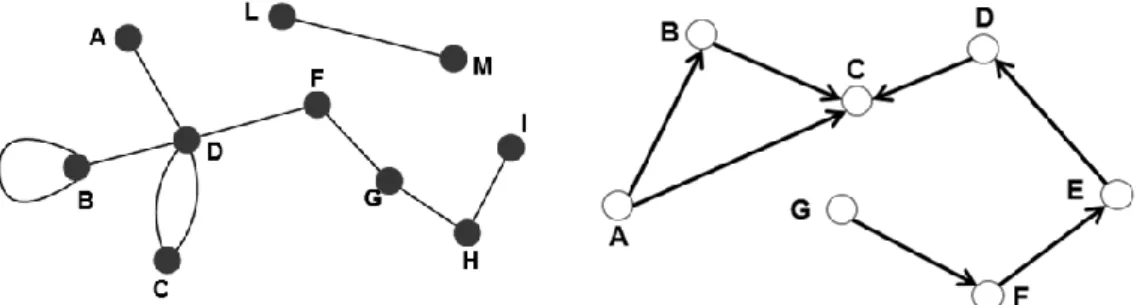
The network-graph is termed as a directed network, when the edges among the nodes are directed meaning that the connection among the nodes are form one side (directional) or from both sides (bidirectional) and the edges of that network is called directed edges. An example of directed network include citation networks, and the WWW. The network is described as undirected if the direction of the edges are unimportant and are only for connecting the nodes. The aviation network, actor network are examples of undirected networks. The figure 2.2 is an example of the two types of the network.

(16)

The black and white circles indicated the nodes both networks while the letters

indicates the label of the nodes: a, b and so on. The figure on the left shows an undirected network, with N=10 and L=10. While the figure of on the left represents directed network, with N=7 and L=7. It is important to note that lines represent the edge and arrows indicate the direction of the relationship. Directed network can also have a node which has an edge to itself called loop.

2.2.2. Network properties and metrics Paths

Physical objects are characterized by the distance between them. For instance the distances between houses in neighborhood, however, when it comes to the network this phenomena is quite complex (Barabási A. , 2012). For example what is distance between two friends in the face book or any other social platform? In order to find the solution of such kind of problem we have to consider the path length between the two. “Path length is a network metric which is any sequence of nodes in which every consecutive pair of nodes in the network are

connected by an edge” (Barabási A. , 2012). A geodesic path, also called simply a shortest path, is a path between two vertices such that no shorter path exists: Geodesic paths are necessarily self-avoiding. If a path intersects itself then it contains a loop and can be shortened by removing that loop while still connecting the same start and end points, and hence self-intersecting paths are never geodesic paths. The diameter of a graph is the length of the longest geodesic path between any pair of vertices in the network for which a path actually exists. (If the diameter were merely the length of them longest geodesic path then it would be formally infinite in a network with more than one component if we adopted the convention above that vertices connected by no path have infinite geodesic distance. One can also talk about the diameters of the individual components separately, this being a perfectly well-defined concept whatever convention we adopt for unconnected vertices.)

Connectivity

The key utility of networks is that they are built to ensure connectedness: they must be capable of establishing a path between any two nodes in a network. A network is said being connected if there is a path between any two pairs of nodes in the network. In disconnected network its parts are called components or clusters. “A component is a subset of nodes in a network, so that there is a path between any two nodes that belong to the component, but one

(17)

cannot add any more nodes to it that would have the same property” (Barabási A. , 2012, p. 39).s

Components

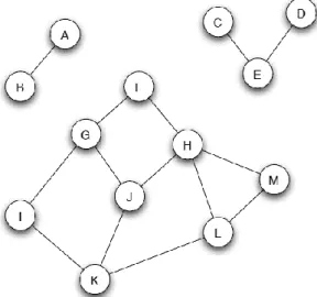
Components. Figures 2.5 make visually apparent a basic fact about disconnected graphs: if a graph is not connected, then it breaks apart naturally into a set of connected “pieces," groups of nodes so that each group is connected when considered as a graph in isolation, and so that no two groups overlap. In Figure 2.5, we see that the graph consists of three such pieces: one consisting of nodes A and B, one consisting of nodes C, D, and E, and one consisting of the rest of the nodes. The network in Figure 2.6 also consists of three pieces: one on three nodes, one on four nodes, and one that is much larger.

Figure 2.3: Example of network components in an undirected network. Centrality

Having seen properties of some networks, it is intuitively clear that some nodes are more essential than others. In transportation networks some nodes are more highly connected than others. The concept of central nodes and edges is intimately linked to the study of network resilience, robustness and susceptibility to targeted attacks. Presumably, failure of central nodes has more dramatic consequences than failure or peripheral nodes or edges.

Degree

The number of edges connected to a nodes is called degree. We will denote the degree of node i by ki. For an undirected graph of n nodes the degree can be written in terms of the

(18)

𝐾𝑖 = ∑ 𝐴𝑖𝑗 𝑛

𝑗=1

Node degrees are more complicated in directed networks. In a directed network each node has two degrees. The in-degree is the number of ingoing edges connected to a node and the out degree is the number of outgoing edges. Bearing in mind that the adjacency matrix of a directed network has element Aij = 1 if there is an edge from j to i, in- and out-degrees can

be written 𝐾_𝑖𝑖𝑛 _{= ∑} _𝐴 𝑖𝑗 𝑛 𝑗=1 𝐾𝑗 𝑜𝑢𝑡 _{= ∑} _𝐴 𝑖𝑗 𝑛 𝑖=1 Hub and Authorities

In the case of directed networks, there is another twist to the centrality measures introduced in this section. So far we have considered measures that accord a node high centrality if those that point to it have high centrality. However, in some networks it is appropriate also to accord a node high centrality if it points to others with high centrality. Thus there are really two types of important node in these networks: authorities are nodes that contain useful information on a topic of interest; hubs are nodes that tell us where the best authorities are to be found. An authority may also be a hub, and vice versa: review articles often contain useful discussions of the topic at hand as well as citations to other discussions. Clearly hubs and authorities only exist in directed networks, since in the undirected case there is no distinction between pointing to a node and being pointed to. However this network which is understudy has no authorities since there is no data about the communication of the nodes in the network.

Closeness Centrality

An entirely different measure of centrality is provided by the closeness centrality, which measures the mean distance from a node to other vertices. In Section 6.10.1 we encountered the concept of the geodesic path, the shortest path through a network between two vertices. Suppose dij is the length of a geodesic path from i to j, meaning the number of edges along the path. Then the mean geodesic distance from i to j, averaged over all vertices j in the network, is

ℓ_𝑖 = 1

𝑛∑ 𝑑𝑖𝑗

.

(19)

This quantity takes low values for vertices that are separated from others by only a short geodesic distance on average. Such vertices might have better access to information at other vertices or more direct influence on other vertices. In a social network, for instance, a person with lower mean distance to others might find that their opinions reach others in the

community more quickly than the opinions of someone with higher mean distance. In calculating the average distance some authors exclude

Betweenness Centrality

A little bit more sophisticated is the concept of betweenness centrality. This measure tries to capture the situation illustrated in Fig. 1.19 in this network, one of the nodes connects two parts of the network. Clearly this node is important in the sense that if it were removed it would disconnected the whole network. Note that a high degree is not required for this function, in fact in the example network other nodes have a more important role. The way to capture this type of centrality is betweenness: the fraction of shortest paths that pass through a node. Bi the subset of shortest paths that pass through node i. The betweenness

𝑏𝑖 = 𝐵_𝑖

𝑆

Is defined as the number of elements in the set B by the total number of shortest paths in the Network S.

Adjacency Matrix

There are a number of different ways to represent a network mathematically. Consider an undirected network with n vertices and let us label the vertices with integer labels 1 . . . n, as we have, for instance, for the network in Fig. 6.1a. It does not matter which vertex gets which label, only that each label is unique, so that we can use the labels to refer to any vertex

unambiguously. If we denote an edge between vertices i and j by (i,j) then the complete network can be specified by giving the value of n and a list of all the edges. For example, the network in Fig. 6.1a has n = 6 vertices and edges (1,2), (1,5), (2,3), (2,4), (3,4), (3,5), and (3,6). Such a specification is called an edge list. Edge lists are sometimes used to store the structure of networks on computers, but for mathematical developments like those in this chapter they are rather cumbersome.

(20)

A better representation of a network for present purposes is the adjacency matrix. The adjacency matrix A of a simple graph is the matrix with elements Aij such that

Aij= { 1 if there is an edge between vertices 𝑖 and 𝑗,

0 otherwise".

Two points to notice about the adjacency matrix are that, first, for a network with no self-edges such as this one the diagonal matrix elements are all zero, and second that it is symmetric, since if there is an edge between i and j then there is an edge between j and i. (Newman M. , Networks: an introduction, 2010)

2.3. Graph clustering and Modularity

The problem of clustering groups in a graph has been a very popular problem in recent years. Clustering groups has many real world applications resulting in the interest of many interdisciplinary fields of research. Detecting communities through community structure is used to find naturally forming groups of actors, represented by vertices that have more interactions, represented by edges, inside the group that they belong to than with the rest of the network. These groups of vertices are commonly referred to as clusters, c. In the context of social network analysis we also refer to these clusters as communities.

A partition, P of a graph, G, is set of clusters where each node is assigned to one cluster. A covering, C, is set of clusters where each node belongs to a minimum one cluster but may belong to multiple. Many of the definitions will be presented for discovering and evaluating partitions and then later are expanded for coverings.

(21)

For successful detection of viable partitions it is necessary that the graph, and thus the network, must be sparse. That is, if the size of the network is n and the number of relations in the network, m, then n >> m, where >> indicates that the number of edges is significantly smaller than the number of vertices. In community detection we expect that as our

communities we use grow in size that m 2 O (n), otherwise more applicable methods would be in the field of research of data clustering. Real networks are known to be sparse and social networks are expected to be sparse.

2.3.1. Community Detection and its algorithm

We now turn to the topics that will occupy us for much of the rest of the chapter, graph

partitioning and community detection.Both of these terms refer to the division of the vertices

of a network into groups, clusters, or communities according to the pattern of edges in the network. Most commonly one divides the vertices so that the groups formed are tightly knit with many edges inside groups and only a few edges between groups. Consider, for instance, which shows patterns of collaborations between scientists in a university department. Each vertex in this network represents a scientist and links between vertices indicate pairs of scientists who have coauthored one or more papers together.

As we can see from the figure, this network contains a number of densely connected clusters of vertices, corresponding to groups of scientists who have worked closely together. Readers familiar with the organization of university departments will not be surprised to learn that in general these clusters correspond, at least approximately, to formal research groups within the department. But suppose one did not know how university departments operate and wished to study them. By constructing a network and then observing its clustered structure, one would be able to deduce the existence of groups within the larger department and by further

investigation could probably quickly work out how the department was organized.

Thus the ability to discover groups or clusters in a network can be a useful tool for revealing structure and organization within networks at a scale larger than that of a single vertex. In this particular case the network is small enough and sparse enough that the groups are easily visible by eye. Many of the networks that have engaged our interest in this book, however, are much larger or denser networks for which visual inspection is not a useful tool. Finding clusters in such networks is a task for computers and the algorithms that run on them.

(22)

PARTITIONING AND COMMUNITY DETECTION

There are a number of reasons why one might want to divide a network into groups or

clusters, but they separate into two general classes that lead in turn to two corresponding types of computer algorithm. We will refer to these two types as graph partitioning and community detection algorithms. They are distinguished from one another by whether the number and size of the groups is fixed by the experimenter or whether it is unspecified.

Graph partitioning is a classic problem in computer science, studied since the 1960s. It is the problem of dividing the vertices of a network into a given number of non-overlapping groups of given sizes such that the number of edges between groups is minimized.

The important point here is that the number and sizes of the groups are fixed. Sometimes the sizes are only fixed roughly— within a certain range, for instance—but they are fixed

nonetheless. For instance, a simple and prototypical example of a graph partitioning problem is the problem of dividing a network into two groups of equal size, such that the number of edges between them is minimized. Graph partitioning problems arise in a variety of

circumstances, particularly in computer science, but also in pure and applied mathematics, physics, and of course in the study of networks themselves. A typical example is the numerical solution of network processes on a parallel computer.

(23)

The Kernighan-Lin algorithm, proposed by Brian Kernighanand Shen Lin in 1970, is one of the simplest and best known heuristic algorithms for the graph bisection problem. The algorithm is illustrated in Fig. 11.2. We start by dividing the vertices of our network into two groups of the required sizes in any way we like. For instance, we could divide the vertices randomly. Then, for each pair (i, j) of vertices such that i lies in one of the groups and j in the other, we calculate how much the cut size between the groups would change if we were to interchange i and j, so that each was placed in the other group. Among all pairs (i, j) we find the pair that reduces the cut size by the largest amount or, if no pair reduces it, we find the pair that increases it by the smallest amount. Then we swap that pair of vertices. Clearly this process preserves the sizes of the two groups of vertices, since one vertex leaves each group and another joins. Thus the algorithm respects the requirement that the group stake specified sizes.

Figure 11.2: The Kernighan-Lin algorithm. (a) The Kernighan-Lin algorithm starts with any division of the vertices of a network into two groups (shaded) and then searches for pairs of vertices, such as the pair highlighted here, whose interchange would reduce the cut size between the groups. (b) The same network after interchange of the two vertices.

(24)

Chapter 3: Research Method

The main purpose of this chapter is to present key research methods followed for the collection, analysis, visualization and the interpretation of dataset used for this study.

The research study is using both quantitative and qualitative research methods because theoretically network science and social network analysis is greatly influenced by social science specially sociology. The first studies in social network where in qualitative in nature and is also used in contemporary researches by some researchers (Waldstrøm, 2003). The main goal of this study is to identify and sufficiently measure the social ties among the nodes in the network under study.

The study of relationship or social ties among individuals in a community or in organization is subjective by nature and difficult to be quantified. For that reason the research is partially dealing with qualitative research methods and partly quantities research methods were we are going to calculate all the fundamental metrics of the network including the centrality, network diameter, graph density, modularity, etc.

The survey was conducted to collect all the necessary data and information for one month period of time. The most commonly used data collection technique used for this kind of research is self-reporting questionnaire and it was given to 151 respondents from the University of the Eight Major Faculties.

Research conducted in the field of network science specially is social networks usually interested in social ties and the type of relationship among the individual in that specific network. The aim of this study is to find this social ties, understand network structure and the communities, to discover the giant components and the hubs, to measure the centralities and determine who is important in this network and eventually visualize the network using visualization tools.

To find all these requirements several attributes of the respondents were interested in the questionnaire. The first part of questionnaire name, surname, title, and the faculty of each respondent were asked. The reason behind this was to find the list of nodes and their attributes.

(25)

The 151 individuals surveyed are members of 8 major faculties of the institute namely:  School of foreign language,

 Law,

 Vocational School,

 Engineering and Natural Science,  Communication,

 Art and Design,  Applied Science,

 Economy, Administration and Social Science

Figure 3.1: shows the percentage of respondents according to their faculties.

28% of survey was conducted in was Eng. & Natural Science Faculty, while 18% of respondents were in the Law Faculty, another 18% was from Communication Faculty, 12% from Vocational School, 9% from “Economy, Administration and Social Science, 8% from Applied Science, while 1% was from Administration and another 1% was from School of Foreign Languages.

(26)

The respondents have six different academic titles including  Research Assistant  Instructor  Lecturer  Assistant Professor  Associate professor  And Professor

Figure 3.2: Shows the respondent titles

Gender attribute was not included during the data collection period but later on we added it as an extra data in order to obtain additional information. 53% of respondents were female while the male respondents where 47%.

Figure 3.3: shows the percentage of male and female respondents

The second part of the questionnaire was concerning finding who socializes with who finding this information is important for mapping the social ties among the individuals in the network to create the number of edges (connections) in the network. In order to find this information the following question was asked in the questionnaire.

Please state those people who you socialize with within the university?

After collecting all the questionnaires the data was compiled into excel sheet by listing all nodes with their attributes into worksheet and the edges (link) into separate worksheet.

(27)

2.1. Nodes

In many social network analysis, different social entities are studied and then analyzed ranging from individuals, groups, departments, objects, etc. however in this intra-organizational network the entities the entities we are going to analyze will be individuals specially the academic staff of knowledge institute which will the nodes in the network terminology.

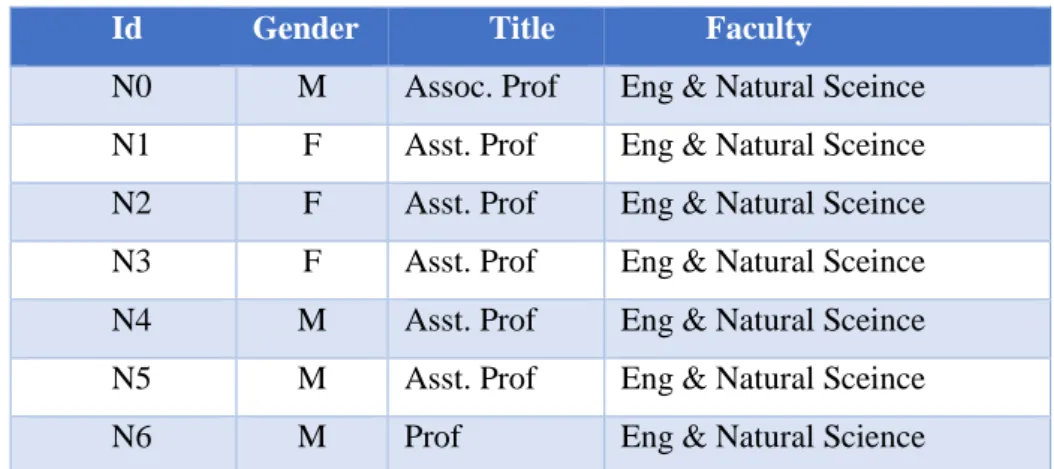
The following table indicates a sample of how the list nodes were created in the dataset using excel spreadsheet however the names of people in the network was purposefully omitted to ensure privacy of the individuals under the study.

Table 3.1: sample of node list 2.2. Edge

Since the social ties (edges) among the nodes in network are the fundamental unit of analysis, the most important task in data collection was to find the exact relationship among the nodes in the network. However finding the exact social ties is not easy as finding nodes because some people might miss-understand the kind of relationship that were aske or might interpret in another way which is not intended or might consider it as privacy. Yet the result is satisfactory to reveal the intended purpose of research and to understand the overall structure of the network.

From Title Faculty To Title Faculty

n0 Assoc. Prof Eng. & Natural Science n21 Inst Eng. & Natural Science n0 Assoc. Prof Eng. & Natural Science n8 Inst Eng. & Natural Science n0 Asst. Prof Eng. & Natural Science n4 Asst. Prof Eng. & Natural Science n1 Asst. Prof Eng. & Natural Science n18 Prof Eng. & Natural Science n1 Asst. Prof Eng. & Natural Science n69 Prof. Eng. & Natural Science n1 Asst. Prof Eng. & Natural Science n8 Inst Eng. & Natural Science n3 Asst. Prof Eng. & Natural Science n81 Asst. Prof Eng. & Natural Science

Table 3.2: sample of how the edges were created.

Id Gender Title Faculty

N0 M Assoc. Prof Eng & Natural Sceince N1 F Asst. Prof Eng & Natural Sceince N2 F Asst. Prof Eng & Natural Sceince N3 F Asst. Prof Eng & Natural Sceince N4 M Asst. Prof Eng & Natural Sceince N5 M Asst. Prof Eng & Natural Sceince N6 M Prof Eng & Natural Science

(28)

The following table indicates a sample of how the list nodes were created in the dataset using Microsoft Excel which is popular spreadsheet family of software and a member of Microsoft office suit. Spreadsheets allow you to keep track of data, create charts based from data, and perform complex calculations. (Bernard Poole, 2002)

After the list nodes and edges were created in excel worksheet the two files were converted into csv format and imported into Gephi. Gephi is an open source network exploration and manipulation software. Developed modules can import, visualize, spatialize, filter, manipulate and export all types of networks. (Mathieu Bastian, 2009).

2.3. Tools

The Gephi software is used for the visualization of network using different network layout. The most widely used layout in this research is Yifan Hu proportional. The Yifan Hu Multilevel layout algorithm is an algorithm that brings together the good parts of force-directed algorithms and a multilevel algorithm to reduce algorithm complexity. This is one of the algorithms that works really well with large networks (Khokhar, 2015).

The visualization tools which is used in Gephi also includes coloring the nodes using various node attributes and changing the size of nodes according to different network metrics such degree centrality etc.

Figure 3.5: Network overview showing eight faculties with different colors and size according to the degree centrality

Moreover a list of metrics, filters and timelines of graph is used for Gephi including network diameter, graph density, graph modularity, connected components in the graph and so on. The visualization of the network graph is partly used Cytoscape. Cytoscape is an open source software platform for visualizing molecular interaction networks and biological

(29)

pathways and integrating these networks with annotations, gene expression profiles and other state data. Although Cytoscape was originally designed for biological research, now it is a general platform for complex network analysis and visualization. (KristinaHanspers, 2013)

(30)

Chapter 4: Result and Discussion

4.1. Introduction

This network under study is small network. It contains 151 nodes and 413 edges. The first section of this chapter deals with the egocentric (individual level) analysis. Egocentric analysis makes discussion on the basic network metrics using centrality measures including degree, betweenness and closeness centrality. It will also study the cluster coefficient, network diameter, graph density. The second section of the chapter deals with socio-centric (group level) analysis by discussing the number of communities in the network using modularity analysis, number of connected components, hubs, the largest communities, and the strong versus weak ties,

4.2. Overview of the Network

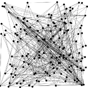
To understand the overview of the network and how the nodes connected. The following figure 4.1. Depicts the first basic visualization the network using Gephi, this figure gives you the big picture of the overall structure of the network without much detail about the network and its character tics. This network represents the social ties among academic staff in knowledge institute. The whole network is one giant connected component.

Figure 4.1: the figure shows general overview of the network. This figure is generated using the default layout of Gephi visualization software.

(31)

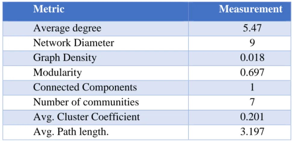
Table 4.1 summarizes the basic metrics of the network including average degree, network diameter, and graph density, modularity, and connected components, number of communities, cluster coefficient and average path length.

Metric Measurement Average degree 5.47 Network Diameter 9 Graph Density 0.018 Modularity 0.697 Connected Components 1 Number of communities 7

Avg. Cluster Coefficient 0.201

Avg. Path length. 3.197

Table 4.1: overall basic metrics of the network. 4.3. Small world effect and scale free networks

One interesting discussions that this network exhibits is the small world phenomena which is specific to scale free networks where most nodes are not neighbors of one another,

but the neighbors of any given node are likely to be neighbors of each other and most nodes

can be reached from every other node by a small number of hops or steps. While at the same

time the level of transitivity, or clustering is relatively high. İn this case the average path

length which is the shortest paths between all pairs of nodes is 3.197 which indicates the any chosen node from network can reach any other node with only three intermediate connections. While the diameter of a network which is the maximum shortest path in the network 9. In other words, it is the largest distance recorded between any pair of nodes is 9 which shows this network have similar characteristics with other real world networks.

4.4. Degree Distribution

The main difference between a random and scale-free network comes in the tail of degree distribution. Random network and scale free network exhibit totally different structure and behavior. In random network the degree distribution should follow a poison distribution, also in random networks the highly connected nodes or hubs are effectively forbidden while scale free network follow the power law which is rich get richer phenomena (Barabasi, 2014).

(32)

Figure 4.2: Degree Distribution of the network

This graph conforms the scale free network which indicates it has real network behavior. Scale free networks are popular most of the nodes in the network have low degree but few nodes are having degree which greatly exceed the average and those nodes are often become the hubs of the network which serve a specific purpose for the network. The average degree of this network is 5.47. It indicates that this network is showing the small world phenomena of the scale free networks. In the language of statistics we say that the degree distribution is right skewed as the one shown fig 4.2.

4.5. Degree Distribution of Random Network

To make sure the scale freeness of the network we have generated a random network using Gephi with the same number of nodes as the real network to compare the two networks properties. The graph in Figure 4.2. Confirms the degree distribution of random network is the binomial form (Barabasi, 2014). And proves our network is not a random network.

(33)

4.6.Node attributes.

The members of the network are from seven major faculties of the knowledge institute. The nodes in the dataset have the following attributes: a node id, faculty, title and gender. To understand the network in organizational context we have to look on how the network is distributed according to different faculties, titles and then the gender. Primarily we need see how the node associates or socializes with other nodes by observing the edges within the faculty. Table 4.2 shows the number of nodes and edges for each department.

Faculty Percen tage # of Nodes # of edges Average Degree Av.Path Length Module Diameter

Eng. & Natural Science 27.81 42 90 4.286 2.4 7

Law 17.99 27 62 4.593 2.050 5

Communication 17.88 27 89 6.693 2.188 5

VS 11.92 18 53 5889 2.098 4

Applied Science 8.61 13 18 2.769 1.743 4

"Eco, Admin & Social Science"

8.61 13 0 0 NaN 0

Art and Design 5.3 8 0 0 NaN 0

Table 4.2: shows how nodes are distributed according to different faculties.

The faculty of Eng. & Natural Science is most dense and highly connected faculty internally containing 42 nodes and 90 internal edges. Comprising 27.81% of the network with average degree 4.286 while the second populated faculties are Law and communication faculties with 27 nodes, 62 internal edges and 27 nodes, 89 internal edges respectively. Together making 35.87% of the network. The Applied Science faculty contains 13 nodes and 18 internal edges which makes it weakly connected faculty to itself compared to previously mentioned faculties. As you can see from above table the faculties of “Eco, Admin & Social Science” and Art and Design are totally two disconnected faculties internally.

The following figure shows how nodes are distributed according to the various faculties using coloring scheme

(34)

Figure4.4: indicates the network layout using color for faculties and size shows the degree of the nodes. The visualization of the network using Force Atlas 2 layout of Gephi, the layout belongs to class of force-directed algorithms in Gephi and is made use of quite often.

The phenomenal insight revealed by the above figure is that Eng. & Natural Science is the most highly connected faculty in the network with 96 internal edges which makes them a separate sub community in the network. There are only two members of faculty which have no edge in to the group.

Figure 4.5: Eng. & Natural Science faculty has the highest number of nodes in the network.

Law, and Communication are also highly connected within themselves and each creates itself as a sub community in the network. Conforming the homophily and assortative mixing. For instance, if the network resembles a system of friendships among students we can investigate how properties of individual nodes such as race, sex, age, nationality determine a networks connectivity.

However on the other hand Vocational School and the faculty of Applied Science are weakly connected according to their faculties. But the two faculties are strongly connected to each other with few nodes from social science and art and design and two nodes from law and natural science faculty. They consider themselves as one sub interconnected community. One possible reason of these interconnectivity could be that there are more common courses which is offered between the two faculties most of the academician thought in both faculties.

(35)

Figure 4.6: Vocational School and faculty of applied science with few other nodes create an interconnected cluster.

One more interesting notion is that faculty of “Economy, Administration and Social Science” and the faculty of Art and Design, are total disconnected and defragmented internally as faculty and both are dispersed to the other faculties by not considering themselves as a community or cluster.

…… …

Figure 4.7: shows Economy, Administration and Social Science color coded with blue and Art and Design colored with red, the two faculties are internally defragmented.

Again let us look how whether the professional title has effect on how the people in this network socialize with each other. As can be seen the following figure generally has no great effect on how people associate with each other the network. You can observe the different titles are evenly distributed in the whole network except a clique research assistants that somehow more connected to each other making them a small cluster. It looks that they consider themselves as peer group which may the cause that creates this effect.

(36)

Figure 4.8: showing how the nodes are connected according to title attribute of the node. The figure uses Yifan hu layout algorithm color coded with titles.

If you look how the network is distributed according to gender we will find that it is again evenly gender is evenly distributed in the network as the following figure indicates

Figure 4.9: this visualization of network is generated using Force Atlas 2 color coded with gender the dark green indicating Female and dark gold showing male nodes

4.7. Network Centrality

The concept of centrality has been examined in various research domains including network science. Essentially, centrality addresses the question “who are the most important or central nodes in the network?” The concept of centrality measure was originally used in fields studying human communication and social networks and later used in this new field of network science ( (Ron Hagan, 2015).

The word central varies by context and purpose however we are going to user both local measure using degree centrality and relative to rest of the network using closeness centrality, eigenvector and betweenness centrality.

(37)

4.7.1. Degree centrality

The most basic centrality measurement of a network is degree centrality which is number of edges connected to a node. When the network is a directed network like this network, we have to look both in and out degrees of the nodes. The in degree indicates the number of individuals who are interested to socialize with that specific person. While the out degree indicates the number of people in which particular person choses to socialize with. In our study we are much interested the number of in degrees as they point out the number people who have interest for the same person. This is the same with what happen when ranking pages by search engine which is called page ranking where a webpage is important if it is pointed to by other important pages. (Amyn.langville, 2009)

Figure 4.10: The network graph shows the degree centrality of the network with size of the node while the color indicated the faculty of the node.

If you look closer to the degree centrality you will recognize that the communication faculty have highest nodes with highest degree centrality compared to the other faculties. Thus communication faculty is highly connected component in this network. However most of those connection are internal which means the faculty has less communication with other faculties causing to have less influence on the other faculties. In contrast the “Economy, Administration and Social science” and Art& Design faculties have almost zero connection within their faculties while they are dispersed throughout the network. In this case we were

(38)

expecting they will have higher degree centrality however the graph shows they have little significance with degree centrality.

Several nodes play an important role according to the degree centrality in this network. Top ten nodes with the highest degree centrality made the central hubs of the network

4.7.2. Analysis of the Hubs

There are two important types of nodes in most network these are the authorities which are nodes that contain significant information about the topic of interest like an important article. And hubs which with high degree centrality nodes that tells where the authorities are found. This network contains no authorities because we are not dealing with communicating information rather we are dealing with social ties so we are only discussing the hubs in this case.

Figure 4.11: Largest hubs in the network three from communication department five from VS and two from applied science faculty.

This above figure shows the assortativity of this network. In assortative networks hubs tend to connect to other hubs, hence the higher is the degree k of a node, the higher is the average degree of its nearest neighbors (Barabasi, 2014). The following table lists the hubs of the network. Therefore it seems reasonable to suppose that individuals who have connections to many others might have more influence, more access to information, or more prestige than those who have fewer connections (Newman M. E., 2010).

Those hubs hold the network together. For example if n49 is removed from the network it obvious that the network will fall apart into separate disconnected networks.

(39)

Node Id Faculty Title Modularity Gender Degree

n62 Communication Asst. Prof 7 F 25

n65 Communication Lect 7 F 21

n42 VS Lect 3 M 18

n61 Communication Asst. Prof 7 F 17

n74 Applied Science Asst. Prof 3 F 16

n48 VS Lect 3 F 16

n45 VS Lect 3 M 16

n49 VS Asst. Prof 3 F 14

n75 Applied Science Prof 5 M 14

n50 VS Lect 3 F 14

Table 4.3: The table shows top 10 nodes with highest degree centrality

The in-degree and out-degree for the degree centrality gives you an extra information about the importance of the node. For instance the number of citations a paper receives from other papers, which is simply its in-degree in the citation network, gives a crude measure of whether the paper has been influential or not and is widely used as a metric for judging the impact of scientific research or web page ranking the page with most inward edges usually ranked first. Hence in social settings the in-degree shows more importance and influence then the out-degree.

Nod e ID

Faculty Title Modularit

y Class Gende r In degree Out degree degree

n74 Applied Science Asst. Prof 3 F 11 5 16

n62 Communication Asst. Prof 7 F 9 16 25

n48 VS Lect 3 F 9 7 16

n84 Eng. & Natural Science

Assoc. Prof 6 M 9 0 9

n64 Communication Lect 7 M 8 5 13

n69 Communication Prof 4 M 8 4 12

n68 Communication Asst. Prof 7 M 8 4 12

n115 Applied Science Lect 3 F 8 0 8

n49 VS Asst. Prof 3 F 7 7 14

n57 Communication Asst. Prof 7 F 7 6 13

Table 4.4: Top ten nodes shown with their in and out degree centrality to reveal extra information

If you look n84 in the above table is a member of Eng. & Natural science faculty. It was not part of survey. It has zero out degree centrality or its social ties are unknown. Furthermore he is not top 10 list with highest degree centrality. However when we look specifically to its

(40)

in-degree centrality we find that n84 is very important person inside the network. It has 9 connection pointing toward it.

Thus becoming the second highest in-degree centrality with n62 after n74 which is having the first rank with 11 incoming edges. We expect if the person was a part of the survey we could have seen a bigger picture of how it is influencing the network.

4.7.3. Betweenness centrality

Betweenness centrality measures the extent to which a node lies on paths between other nodes hence connecting various nodes, communities and clusters within the network or with other network. Betweenness centrality indicates how much the person is able to influence communication between other persons (Newman M. E., 2010).

Figure 4.12: shows the betweenness centrality with size and node faculty with color

Previously when we were discussing the degree centrality we have seen generally the communication department which was internally highly connected has the overall maximum degree centrality were almost 25% of the highest degree where from that department. However when we look betweenness centrality you will find the Vocational school together with applied science department have the highest betweenness centrality making them the bridges between these network except node n62 in communication faculty which proves to be the most important node in the network both according to degree centrality and betweenness centrality.

(41)

Node Id

Faculty Node Title gender Modularit

y Class

Betweenness Centrality

n62 Communication Asst. Prof F 7 692

n49 VS Asst. Prof F 3 608

n42 VS Lect M 3 410

n48 VS Lect F 3 299

n46 VS Asst. Prof M 3 254

n75 Applied Science Prof M 5 250

n54 VS Lect M 3 235

n77 Applied Science Prof M 3 228

n69 Communication Prof M 4 211

n22 Eng. & Natural Science

Asst. Prof F 6 210

Table 4.5: top 10 nodes with highest betweenness centrality sorted descending order according to their betweenness centrality

The removal of one or two of those top 10 highest betweenness nodes can lead the network to disintegrate and fall into parts. n62, n49 and n48 from the above table are also members of the top 10 with highest degree centrality. These three nodes play and important position in the network since they are having highest centrality in both degree and betweenness centrality.

4.7.4. Closeness centrality

A different measure of centrality is the closeness centrality which measures the mean distance of node from other nodes in the network. Nodes with high closeness centrality have a better chance to access information from other nodes easily. On the contrary they can spread their opinion to the nodes more quickly compared to other nodes. Thanks to their high degree centrality.

(42)

Figure 4.13: shows the social graph with faculties (color coded) and betweenness centrality (size coded)

If you look the overall degree centrality you will find that communication department has the highest degree centrality in the network. But if you look the betweenness centrality you are going find that VS and Applied science together have the overall betweenness centrality. Furthermore when we look the closeness centrality what we are observing is that it is somehow evenly distributes among the various faculties apart from “Economy, Admin and Social science and Art and Design. Both of these faculties are loosely connected internally. The following table depicts the top 10 nodes with highest closeness centrality. It is important to note that none of these 10 are in the list of top 10 list in either degree centrality or closeness centrality.

Node Id Faculty Title gender Closeness

centrality

n36 Law Asst. Prof F 1.0

n63 Communication Lect F 1.0

n19 Eng. & Natural Science Asst. Prof M 1.0 n16 Eng. & Natural Science Asst. Prof M 1.0

n52 VS Lect F 1.0

n38 Law Res. Asst F 0.78

n14 Eng. & Natural Science Asst. Prof M 0.74

n5 Eng. & Natural Science Asst. Prof M 0.68

Table 4.6: top 10 nodes with highest closeness centrality sorted descending order according to their closeness centrality

4.8. Network Structure and Modularity analysis.

Community structure is the main focus of this thesis and will be addressed in the following section. In this thesis a general definition of community structure introduced by Newman (Newman M. , A measure of betweenness centrality based on random, 2005) is used, namely “The division of network nodes into groups within which the network connections are dense, but between which are sparser”.

We now turn to the topics that will occupy us for much of the rest of the chapter, graph partitioning and community detection. Both of these terms refer to the division of the vertices of a network into groups, clusters, or communities according to the pattern of edges in the

(43)

network. Most commonly one divides the vertices so that the groups formed are tightly knit with many edges inside groups and only a few edges between groups (Newman M. E., 2010). An example of a network with community structure is depicted in Figure 4.14. Nodes in a community should share more connections with each other than with nodes in other communities. In the example, nodes within a community are completely connected meaning that all possible edges within

Figure 4.14: Example of a network with 8 communities, highlighted by the dashed circles this visualization is generated with Cytoscape. The good thing of this visualization is that each community

is separated from the other and easily can be visualized.

Formally the institute’s structure divides into Faculties which in turn is divided into departments each department contains employees with specific profession. However the social ties among employees of any organization normally do not follow the same rule when it comes to the socializing with other members in the group. The above figure demonstrates how the academic staff of knowledge institute and interconnected with eight non formal groups.

Figure 4.15: shows the modularity and structure of the network which is divided into eight unique communities color coded with modularity

(44)

Using fast unfolding algorithms which attracted much interest in recent years due to the increasing availability of large network data sets and the impact of networks on everyday life Gephi produces the eight communities

Modularity ID ommunity percentage No of Nodes No of edges Average Degree Av. Path Length Community Diameter 6 21.19 32 71 4.438 2.441 7 3 20.53 31 104 6.774 2.402 5 7 20.53 31 94 6.065 2.187 5 0 11.92 18 44 4.889 2.188 5 4 9.93 15 27 3.6 1.791 4 5 6.62 10 12 2.4 1,612 2 2 4.64 7 14 4 1.5 3 1 4.64 7 8 2.286 1.625 3

Table 4.7: summarizes the general property the eight modules sorted with biggest modules. 4.8.1. Largest Communities

The giant connected component in the network is community 6 which makes 21.19% of the overall network with 32 nodes and 71 edges the longest shortest path of module is 7. İt contains mainly the Engineering and Natural faculty except one nodes from Art & design faculty.

When we perform modularity analysis using Gephi with the resolution of 1, we found eight modules which indicated the total number of community present in the network the largest three communities was further analyzed with only one giant component because all nodes are somehow connected

(45)

The second largest community in this network is community 3 which is 20.53% of the whole network, this sub community contains 31 nodes and 105 edges. This community basically contains two faculties 9 nodes from applied science faculty, 18 nodes from VS, 3 nodes from Art and Design and 1 node from Engineering and Natural Science faculty, The diameter of this community is 5.

Figure 4.17: second largest community of the network

The third largest community in this network is community 7 which is 20.53% of the whole network, this sub community contains 31 nodes and 94 edges the longest shortest path of module is 5. İt contains mainly three faculties 25 nodes from communication faculty, 4 nodes from “Eco, Admin and social network, 3 nodes from Art & design.

Figure 4.18: Third Largest community of the network

4.9. Cluster Coefficient

in social networks a large fraction of triplets are triangles, which means if A is friends with B and C then with a high probability B and C are also friends. So one way of measuring the strength of transitivity of an undirected unweighted network is by the fraction of triangles with respect to the entire set of triplets.

C =3 ∗ #𝑡𝑟𝑎𝑖𝑛𝑔𝑙𝑒𝑠 # 𝑡𝑟𝑖𝑝𝑙𝑒𝑠

(46)

This is called the clustering coefficient. When we compute the clustering coefficient of this network we get C=0.201. This means, given a node and two neighbors, their likelihood of being connected is roughly 20%. This shows the transivity of network is not strong as expected. To find some insight we compare real network with a random network which was generate in Gephi that has the same size and edge density. One such network is the Erdos-Renyi network in which one can specify the average degree <k> and the number of nodes.

So if I have a node and two of its neighbors, the probability of them being connected is entirely random which means its p. So for instance in the network above this would imply that C= 0.201 which is also confirmed by the values shown in Table 4.1. That means, the clustering in the real networks above are much higher than expected by chance. While the random networks’ C= 0.021 which is much less than the real network.

4.10. Hierarchical Clustering

Hierarchical clustering is an agglomerative technique in which we stared the individual level of the nodes and then combined into clusters and visualized in the form of a dendrogram (Newman M. E., 2010). The basic idea behind hierarchical clustering is to define a measure of similarity or connection strength between nodes, based on the network structure, and then join together the closest or most similar nodes to form groups. The hierarchical layout algorithm which is used in Fig. 4.19 is good for representing main direction or flow within a network. Nodes are placed in hierarchically arranged layers and the ordering of the nodes within each layer is chosen in such a way that minimizes the number of edge crossings.

Figure 4.19: ClusterMaker’s Eisen TreeView. The larger image shows the results of hierarchically clustering the nodes. The inset shows the results of hierarchical clustering using a edge.