Approximate Bayes Estimation for Log-Dagum Distribution

Cumhuriyet Science Journal

CSJ

e-ISSN: 2587-246X

ISSN: 2587-2680 Cumhuriyet Sci. J., Vol.40-2 (2019) 477-486

* Corresponding author. Email address: ctanis@selcuk.edu.tr

http://dergipark.gov.tr/csj ©2016 Faculty of Science, Sivas Cumhuriyet University

Approximate Bayes Estimation for Log-Dagum Distribution

Caner TANIŞ1*

, Merve ÇOKBARLI2 , Buğra SARAÇOĞLU1 1,2,3 _{Selçuk University Department of Statistics, Konya, TURKEY}

Received: 18.11.2018; Accepted: 14.01.2019 http://dx.doi.org/10.17776/csj.484730

Abstract.In this article, the approximate Bayes estimation problem for the log-Dagum distribution with three parameters is considered. Firstly, the maximum likelihood estimators and asymptotic confidence intervals based on these estimators for unknown parameters of log-Dagum distribution are constructed. In addition, approximate Bayes estimators under squared error loss function for unknown parameters of this distribution are obtained using Tierney and Kadane approximation. A Monte-Carlo simulation study is performed to compare performances of maximum likelihood and approximate Bayes estimators in terms of mean square errrors and biases. Finally, real data analysis for this distribution is performed.

Keywords: Log-Dagum Distribution Maximum Likelihood Estimation, Asymptotic Confidence Interval, Approximate Bayesian Estimation, Tierneyand Kadane Approximation.

Log-Dagum Dağılımı İçin Yaklaşık Bayes Tahmini

Özet. Bu makalede, log-Dagum dağılımı için yaklaşık Bayes tahmini problemi düşünüldü. İlk olarak,

Log-Dagum dağılımının bilinmeyen parametreleri için en çok olabilirlik tahmin edicileri ve bu tahmin edicilere dayalı asimptotik güven aralıkları oluşturuldu. Ayrıca, bu dağılımın bilinmeyen parametreleri için karesel kayıp fonksiyonu altında yaklaşık Bayes tahmin edicileri Tierney and Kadane yaklaşımı kullanılarak elde edildi. Bu tahmin edicilerin performanslarını, hata kareler ortalaması ve yan bakımından karşılaştırmak için bir Monte-Carlo simülasyon çalışması gerçekleştirilmiştir. Son olarak bu dağılım için gerçek veri analizi gerçekleştirilmiştir.

Anahtar Kelimeler: Log-Dagum dağılımı, En çok olabilirlik tahmini, Asimptotik güven aralığı, Yaklaşık Bayes tahmini, Tierney and Kadane yaklaşımı.

1. INTRODUCTION

Statistical distributions are widely used for analysis of data in the real world. In literature, new statistical distributions have been obtained for modeling data in many areas such as science, engineering, medicine and economy. One of these statistical distributions is the dagum distribution suggested by Dagum [1,2] used for modelling wealth and income data . The cumulative distribution function (cdf) and probability density function (pdf) of a Y random variable having to Dagum distribution with parameters , and  are given by,

(1.1) (1.2)



; , ,  



 



1  



 Y F y y





₁





1 ; , ,      1    Y f y y y

where y0, , 0  , 0   . Domma [3] has introduced the log-Dagum ( LDa ) distribution by 0 using logarithmic transformation, XlnY, of a Y random variable having to Dagum distribution. The cdf and pdf of the log-Dagum (LDa) distribution with  ,  and  parameters are

(1.3)

and

(1.4)

respectively. Where x  ,  , 0 0 and  0. There are few studies about LDadistribution in literature. Domma [4] has proved that the kurtosis for log-dagum distribution depends only on parameter

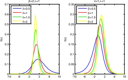
 . Domma and Perri [5] have examined some characteristic properties of this distribution and they have studied about maximum likelihood estimation (MLE) and asymptotic confidence interval for the unknown parameters of log-dagum distribution. The plots of pdf for various parameter values of

LDa



  

, ,



distribution are given in Figure 1.

Figure 1. Density function plots of log-Dagum distribution for different parameter values

In this paper, we consider approximate Bayes estimation problem of unknown parameters



  , ,



for the log-Dagum distribution. This study is organized as follows. In Section 2,

maximum likelihood estimators (MLEs) for unknown parameters of the log-Dagum distribution

and asymptotic confidence intervals based on these estimators are presented. In section 3, Bayes

estimators with Tierney and Kadane approximation under squared loss function for unknown

parameters of the log-Dagum distribution are obtained. In section 4, a Monte-Carlo simulation

study is performed to compare maximum likelihood (ML) and approximate Bayes estimators in

terms of mean square errors (MSEs) and biases. In addition, in this section, a simulation study

based on asymptotic confidence intervals is carried out. A real data application is performed in

section 5. In the last section, the conclusion of this study is given.

-10 -6 -2 2 6 10 0 0.1 0.2 0.3 0.4 0.5 0.6 0.7 x f( x ) =2,=1 =0.5 =1 =1.5 =2 -10 -6 -2 2 6 10 0 0.05 0.1 0.15 0.2 0.25 0.3 0.35 x f( x ) =1,=1 =0.5 =1 =1.5 =2



; , ,  



 



1  x



 X F x e









1 ; , ,    x 1 x   X f x e e

2. ML ESTIMATION and ASYMPTOTIC CONFIDENCE INTERVALS for LOG-DAGUM DISTRIBUTION

Let

X 



X X₁, ₂,...,X_n



be a random sample with size n taken from

LDa



  , ,



distribution. In

that case, the log-likelihood function is given by;

(2.1)

In order to obtain ML estimators, the following likelihood equations should be solved.









1 , , | log 1 i 0 n x i x n e               



(2.2)





_

_

1 , , | 1 0 1 i i x n x i x n e e      _            





(2.3)

(2.4)

The solution of these non-linear equations can be obtained by using iteration methods such as Newton-Raphson method (Domma and Perri [5]).

Large-sample approach is used to obtain asymptotic confidence intervals for unknown parameters. Let ˆ is ML estimator of  and I

 

  ,



  , ,



is Fisher information matrix. In this case, the asymptotic distribution of n    and the Fisher information matrix are



ˆ





ˆ



d



_0, 1

 



n    N I 

 





































2 2 2 2 2 2 2 2 2 2 2 2 , , | , , | , , | , , | , , | , , | , , | , , | , , | x x x E E E x x x I E E E x x x E E E                                                       _   _{ }   _{ }                   _{  }  _{ }  _{ }              _{     }   _{ }  _{ }  _{ }  _{          }             ,

(2.5)

respectively. The elements of fisher information matrix have been obtained by Domma and Perri [5]. The above approaches are used to find the approximate confidence intervals of  , and  parameters. The



1



100% confidence intervals of the , and  parameters are obtained as in equations (2.6),( 2.7) and (2.8).

(2.6)













1 1

, , | log log log 1 log 1 

               



 



 i n n x i i i x n n n x e





_

_

1 1 , , | 1 0 1      _               





 i i x n n i i x i i x n x e x e

 

 

2 2 ˆ ˆ ˆ ˆ ₁                     P z Var z Var

 

 

2 2 ˆ ˆ ˆ ˆ ₁ P_z_ Var      z_ Var  _   

(2.7)

 

 

2 2 ˆ ˆ ˆ ˆ ₁ P_ z_ Var      z_ Var  _   

(2.8)

where diagonal elements of inverse of Fisher information matrix are variances of

ˆ

,

ˆ

and

ˆ

(Domma and Perri [5]).

3. BAYES ESTIMATION for PARAMETERS of LOG-DAGUM DISTRIBUTION

Let X X1, 2,...,Xn be a random sample with size n taken from LDa



  , ,



distribution. It is needed to prior distributions for these parameters to obtain Bayesian estimation of parameters. In this study, it is taken as following gamma priors for unknown

 

, and  parameters.

 

11 1 1 1 , , , 0 d _e e _{e d}   _    _{ (2.9)} (2.10) (2.11)

The joint priors and posterior distributions of ,  and  parameters are,



_{, ,}



     

d1 1 d2 1 d3 1_e e1 e2 e3     _      _       







_{ }

 











0 0 0 | , , , , , , | ( ; , , ) , , ( ; , , ) , , x i i f x x f x k x k x d d d                                 



, (2.12) respectively. Where













1 1 1 ( ; , , ) , , exp 1 exp n n n i i i i i k x        x  x        _ _   

 

 . In this case,

Bayes estimator for any function of ,  and , ( , , ) u    , under squared loss function is as follows.

(2.13)

Where



  

, , | x



is log-likelihood function,

   



, ,



is logarithm of joint prior distribution. It is very difficult to the obtain solution of above Eq. (2.13) in closed form. Some approximate methods for solution of this equation are used. One of these methods is Tierney Kadane’s approximation.

 

2 1 2 2 2 , , , 0    _d _e e  _{e d }

 

3 1 3 3 3 , , , 0    _d  e  _ e e d













        , , | , , 0 0 0 , , | , , 0 0 0

, ,

, ,

|

, , |

             

  

  

  

  

  

                    









B x x

u

E u

x

u

x e

d d d

e

d d d

a. Bayes Estimation with Tierney and Kadane’s Method

Tierney and Kadane’s approximation introduced by Tierney and Kadane [6] to compute integral ratios in bayes analysis has been studied by many authors such as Gencer and Saraçoğlu [7], Howloader and Hossain [8], Mousa and Jaheen [9], Kınacı et al. [10], Tanış and Saraçoğlu [11]. Tierney and Kadane approximation can be summarized as follows.

(2.14)

(2.15)

Where,

   



, ,



is defined as follows.

(2.16)

Bayes estimators with Tierney and Kadane approximation of

u



  

, ,



under squared error loss

function for LDa



  , ,



distribution is obtained as follows









   



 







* * * * , , 0 0 0 , , 0 0 0 1 2 * * ˆ , , , , | det _{ˆ ˆ ˆ ˆ ˆ ˆ} exp , , , , det nI b nI I I I I I I e d d d u E u x e d d d n I I                                _  _ _{    }    _{  }  _      





(2.17)

where



ˆ*, ˆ*,ˆ*



I I I   

and



  ˆ ˆ ˆ_I, _I, _I



maximize



* * *



* ˆ ˆ ˆ , , I I I I   

and

I



  ˆ ˆ ˆ_I, _I, _I



, respectively.



*

and

 are minus the inverse Hessians of



* * *



* ˆ ˆ ˆ , , I I I I   

and

I



  ˆ ˆ ˆ_I, _I, _I



at



ˆ*, ˆ*, ˆ*



I I I   

and



ˆ ˆ ˆ_{, ,}



I I I   

, respectively.

4. SIMULATION STUDY

In this section, a Monte-Carlo simulation study in order to compare the performances of ML estimators and aproximate bayesian estimators according to MSEs and biases for LDa



  , ,



distribution is performed. In addition, in this section, a simulation study based on coverage probabilities (cp) and lengths of asymptotic confidence intervals based on ML estimators is carried out. Firstly, it is needed to generate random samples from LDa



  , ,



distribution for simulation study.

4.1. Random Sample Generation

Inverse conversion method in order to generate random number from LDa



  , ,



distribution is used. Let u state a random number generated from Uniform

 

0,1 . x generated from LDa



  , ,



distribution with inverse conversion method is given as follows.

0 0 1/ 0 1 1 x ln u        _{ }    (3.1)





1





 





, , , , , , |             I x n







 



*   _{, ,} 1_log   _{, ,}    _{, ,} I u I n



, ,

 

1

1 log

   

2

1 log

   

3

1 log

   

1 2 3



where

 

₀, ₀ and



₀ are initial values. (Domma and Perri [7]).

In simulation study, it is generated

N 

5000

samples of sizes n 100,200,500,1000 from



, ,



LDa    distribution with



₀0.43,₀0.2,₀ 0.5



,



₀0.8,₀0.15,₀ 0.3



and



0 0.5,0 0.1,00.7



. The biases and MSEs of ML and approximate bayes estimators for unknown

parameters at different samples sizes as n 100, 200, 500,1000 are given in Table1. In this table, prior values for approximate bayes estimators are d10.01,e10.01 , d20.01,e20.01,d30.01,e30.01

. The results of asymptotic confidence intervals based on ML estimators for unknown parameters of



, ,



LDa    distribution for different samples sizes as n 100,200,500,1000 are presented in Table 2.

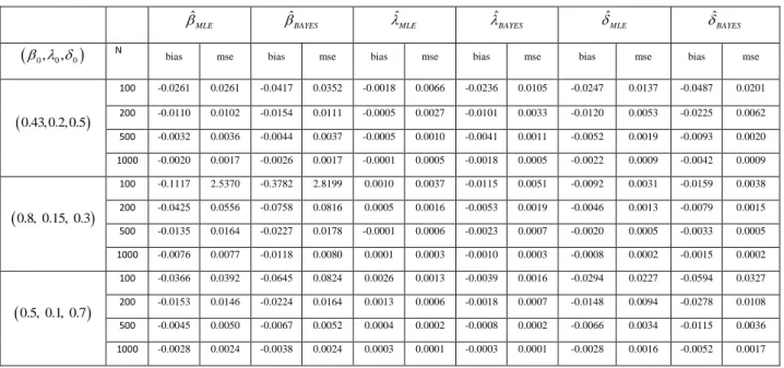
Table 1. Biases and MSEs of MLE and Bayes estimators for LDa



  , ,



ˆ MLE  ˆ BAYES  ˆ MLE  ˆ BAYES  ˆ MLE  ˆ BAYES    0, 0, 0

N _{bias mse bias mse bias mse bias mse bias mse bias mse}

0.43,0.2,0.5 100 -0.0261 0.0261 -0.0417 0.0352 -0.0018 0.0066 -0.0236 0.0105 -0.0247 0.0137 -0.0487 0.0201 200 -0.0110 0.0102 -0.0154 0.0111 -0.0005 0.0027 -0.0101 0.0033 -0.0120 0.0053 -0.0225 0.0062 500 -0.0032 0.0036 -0.0044 0.0037 -0.0005 0.0010 -0.0041 0.0011 -0.0052 0.0019 -0.0093 0.0020 1000 -0.0020 0.0017 -0.0026 0.0017 -0.0001 0.0005 -0.0018 0.0005 -0.0022 0.0009 -0.0042 0.0009 0.8, 0.15, 0.3 100 -0.1117 2.5370 -0.3782 2.8199 0.0010 0.0037 -0.0115 0.0051 -0.0092 0.0031 -0.0159 0.0038 200 -0.0425 0.0556 -0.0758 0.0816 0.0005 0.0016 -0.0053 0.0019 -0.0046 0.0013 -0.0079 0.0015 500 -0.0135 0.0164 -0.0227 0.0178 -0.0001 0.0006 -0.0023 0.0007 -0.0020 0.0005 -0.0033 0.0005 1000 -0.0076 0.0077 -0.0118 0.0080 0.0001 0.0003 -0.0010 0.0003 -0.0008 0.0002 -0.0015 0.0002 0.5, 0.1, 0.7 100 -0.0366 0.0392 -0.0645 0.0824 0.0026 0.0013 -0.0039 0.0016 -0.0294 0.0227 -0.0594 0.0327 200 -0.0153 0.0146 -0.0224 0.0164 0.0013 0.0006 -0.0018 0.0007 -0.0148 0.0094 -0.0278 0.0108 500 -0.0045 0.0050 -0.0067 0.0052 0.0004 0.0002 -0.0008 0.0002 -0.0066 0.0034 -0.0115 0.0036 1000 -0.0028 0.0024 -0.0038 0.0024 0.0003 0.0001 -0.0003 0.0001 -0.0028 0.0016 -0.0052 0.0017

Table 2. Length and cp based on MLE for LDa



  , ,



ˆ MLE  ˆ MLE  ˆ MLE 

  0, 0, 0 n cp length cp length cp length

0.43,0.2,0.5 100 0.9298 0.5739 0.8994 0.2926 0.9456 0.4061 200 0.9446 0.3788 0.9232 0.1982 0.9502 0.2704 500 0.9470 0.2313 0.9388 0.1232 0.9490 0.1662 1000 0.9512 0.1623 0.9444 0.0864 0.9514 0.1161 0.8, 0.15, 0.3 100 0.9310 1.4932 0.8988 0.2216 0.9460 0.2012 200 0.9422 0.8406 0.9260 0.1524 0.9448 0.1370 500 0.9488 0.4928 0.9398 0.0952 0.9538 0.0850 1000 0.9508 0.3424 0.9460 0.0669 0.9518 0.0596 0.5, 0.1, 0.7 100 0.9340 0.6945 0.8974 0.1346 0.9480 0.5367 200 0.9418 0.4516 0.9202 0.0942 0.9502 0.3610 500 0.9494 0.2740 0.9380 0.0593 0.9500 0.2227 1000 0.9506 0.1920 0.9420 0.0418 0.9506 0.1557

According to results of simulation study, it is seen that MSEs and biases values for ML and approximate bayes estimators of parameters are decreases when the number of samples increases. Furthermore, as

sample sizes increases, it is observed that cp approaches to 0.95 and the length of the asymptotic confidence interval decreases as expected.

5. REAL DATA APPLICATION

The data set consist of 76 observations about the life of fatigue fracture of Kevlar 373/epoxy which is considered in this section. These data are obtained by subject to constant pressure at the 90% stress level until all fatigue fracture had failed. (Kharazmi and Saatınık, [12]). This data set have been studied Andrews and Herzberg [13], Barlow et al. [14] and Merovci et. al. [15]. Let x  express data, we consider a transformation with yln( )x _{on Kevlar 373/epoxy data set. Thus, it is obtained y  data.}

Then, new data after transformation is given in Table 3. This data set has been analyzed to compare the log-Dagum distribution with other distributions such as, Normal, Logistic, Laplace, t location-Scale, Extreme Value and Generalized Extreme Value (GEV). Probability density functions of these distributions given by;

 

1



₂



2 : exp , 0, , 2 2 x Normal f x   x    _{ }          

 

2 exp : , 0, , 1 exp x Logistic f x x x   _{ }               _       _{ }  

 

1 : exp , 0, , 2 x Laplace f x   x             

 

1 2 ₂ 1 2 - : , , 0, , 2 x t location Scale f x x   _   _{  }        _ _                 _   _               

 

1

: exp x exp exp x , 0, ,

Extreme Value f x      x            _{  } _{ }       

 









1 1 1 1 : exp 1 1 , 0, , , k k x x GEV f x  k  k   k  x    _{ }             _ _{  }  _          

Table 3. Kevlar 373/epoxy data set -3.6849 -2.4236 -2.4180 -1.3859 -1.1670 -1.0639 -0.7417 -0.5709 -0.5672 -0.4207 -0.3933 -0.3929 -0.3926 -0.2619 -0.1773 -0.1754 -0.1714 -0.1456 -0.1221 -0.0929 -0.0921 -0.0165 0.0472 0.0579 0.0745 0.1598 0.2287 0.2442 0.2612 0.2785 0.3003 0.3039 0.3781 0.3974 0.4529 0.4532 0.5355 0.5460 0.5573 0.5670 0.5736 0.6029 0.6084 0.6153 0.6317 0.6354 0.6356 0.6583 0.6708 0.6955 0.7133 0.7373 0.7464 0.7575 0.7930 0.8092 0.8276 0.8417 0.8531 0.8550 0.9143 0.9266 1.0956 1.1071 1.1841 1.2251 1.2484 1.3200 1.3206 1.3646 1.5701 1.6865 1.6944 1.7101 1.8801 2.2078

MLEs and their standard errors, AIC values for seven distributions are given In Table 5. Moreover, plots fitted to cdfs, reliability functions and pdfs are presented in Figure 4-6.

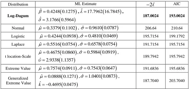
Table 4. Parameter estimates (standard errors) and AIC values for Kevlar 373/epoxy data set

Distribution ML Estimate ₂ AIC

Log-Dagum





ˆ _{0.4248 0.1275}  ,ˆ 17.7962 16.7845





,





ˆ 3.1766 0.5964   187.0024 193.0024 Normal ˆ0.3379 0.1102





, ˆ 0.9610 0.0787





206.64 210.64 Logistic ˆ 0.4244 0.0938





,ˆ 0.4810 0.0469





195.7154 199.1792 Laplace ˆ0.5516 0.0754





,ˆ 0.6578 0.0754





191.7154 195.7154 t location-Scale





ˆ 0.4675 0.0860  ,ˆ 0.5984 0.0919





,





ˆ 2.9338 1.1357  189.7942 195.7942 Extreme Value ˆ0.7574 0.0911





,ˆ 0.7543 0.0647





191.6836 195.6836 Generalized Extreme Value





ˆ 0.0888 0.1271  ,ˆ 1.0401 0.0873





,





ˆ _{0.4695 0.0475} k   187.7040 203.7040

Also, the approximate Bayes estimation values of the unknown parameters of Log-Dagum distribution are obtained as ˆ_BAYES 0.4613 , ˆBAYES 23.2287 , ˆBAYES 3.1277 with prior gamma distribution



d10.01,e10.01,d20.01,e20.01,d30.01,e30.01



.

Figure 2. Fitted cdfs plots for Kevlar 373/epoxy data set

-4 -3 -2 -1 0 1 2 0 0.1 0.2 0.3 0.4 0.5 0.6 0.7 0.8 0.9 1 Data C u m u la ti v e p ro b a b ili ty Data Normal Laplace Logistic t Location-Scale Extreme Value Log Dagum

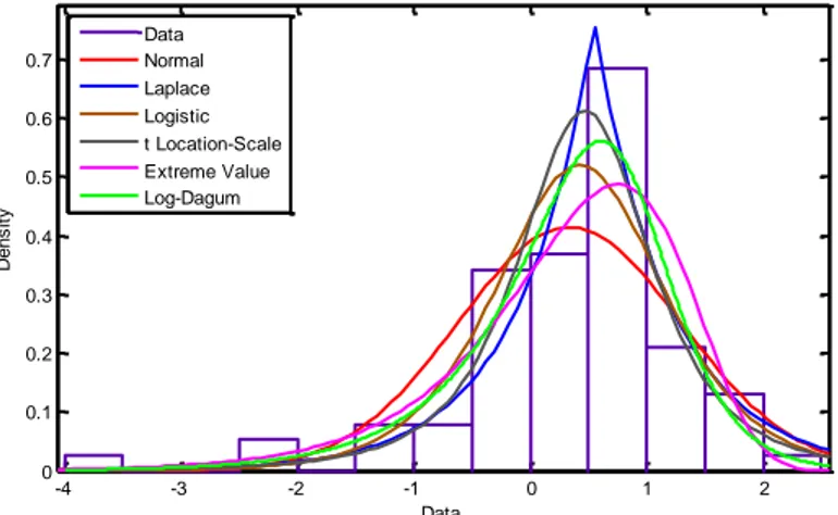
Figure 3. Fitted pdfs plots for Kevlar 373/epoxy data set

6. CONCLUSION

We have analyzed the LDa



  , ,



distribution in terms of estimation of unknown parameters. The approximate Bayesian estimators for unknown parameters of this distribution are obtained. The Bayesian estimators under squared error loss function are found using Tierney and Kadane approximation. The performances of ML and approximate Bayes estimators have been compared with the Monte Carlo simulation study according to MSE and bias criteria. A simulation study based on asymptotic confidence intervals is performed. It is seen that the biases and MSEs of ML and Bayes estimators decrease as sample size increases. It can be concluded that biases and MSEs of these two estimators are very close to each other. In interval estimation based on ML estimators of unknown parameters for theLDa



  , ,



distribution, it is seen that coverage probabilities (cp) approach to 0.95 and length of asymptotic confidence intervals decreases as sample size increases. Furthermore, a real data application is performed in order to show that theLDa



  , ,



distribution can be used in new areas. It is presented a real data set related to the life of fatigue fracture of Kevlar 373/epoxy. We have concluded that the LDa



  , ,



distribution has to best fit between other six distributions (Normal, Logistic, Laplace, t location-Scale, Extreme Value, Generalized Extreme Value) according to AIC and 2 .

REFERENCES

[1] Dagum, Camilo. New model of personal income-distribution-specification and estimation. Economie appliquée, 30-3 (1977) 413-437.

[2] Dagum, C. The Generation and Distribution of Income, the Lorenz Curve and the Gini Ratio, Economie Appliqu ée, 33 (1980) 327-367.

[3] Domma, F., Asimmetrie Puntuali e Trasformazioni Monotone. Quaderni di Statistica, 3 (2001) 145-164.

[4] Domma, F., Kurtosis diagram for the Log-Dagum distribution. Statistica Applicazioni, 2 (2004) 3– 23.

[5] Domma, F., Perri, P. F., Some developments on the log-Dagum distribution. Statistical Methods and Applications, 18-2 (2009) 205-220.

[6] Tierney, L., Kadane, J. B., Accurate approximations for posterior moments and marginal densities. Journal of the american statistical association, 81(393) (1986) 82-86.

[7] Gencer, G., and Saracoglu, B. Comparison of approximate Bayes Estimators under different loss functions for parameters of Odd Weibull Distribution. Journal of Selcuk University Natural and Applied Science, 5-1 (2016) 18-32. -4 -3 -2 -1 0 1 2 0 0.1 0.2 0.3 0.4 0.5 0.6 0.7 Data D e n s it y Data Normal Laplace Logistic t Location-Scale Extreme Value Log-Dagum

[8] Howloader, H.A., Hossain, A. M., Bayesian survival estimation of Pareto distribution of second kind based on failure-censored data, Computational Statistics and Data Analysis, 38 (2002) 301-314. [9] Mousa, M. A., Jaheen, Z. F., Statistical inference for the Burr model based on progressively censored

data. Computers and Mathematics with Applications, 43-10 (2002) 1441-1449.

[10] Kınacı, İ., Karakaya, K., Akdoğan, Y., Kuş, C., Kesikli Chen Dağılımı için Bayes Tahmini. Selçuk Üniversitesi Fen Fakültesi Fen Dergisi, 42-2 (2016) 144-148.

[11] Tanış, C., Saraçoğlu, B., Statistical Inference Based on Upper Record Values for the Transmuted Weibull Distribution. International Journal of Mathematics and Statistics Invention (IJMSI), 5-9 (2017) 18-23.

[12] Kharazmi, O., Saadatinik, A., Hyperbolic cosine-f family of distributions with an application to exponential distribution. Gazi University Journal of Science, 29-4 (2016) 811-829.

[13] Andrews, D. F., and A. M. Herzberg, Prognostic variables for survival in a randomized comparison of treatments for prostatic cancer. Data, (1985) 261-274.

[14] Barlow, R. E., Toland, R. H., and Freeman, T., A Bayes Analysis of Stress-Rupture Life of Kevlar/Eproxy Spherical Pressure Vessels, in Proceedings of the Canadian Conference in Applied Statistics, New York: Marcel Dekker (1984).

[15] Merovci, F., Alizadeh, M., Hamedani, G. G., Another generalized transmuted family of distributions: properties and applications. Austrian Journal of Statistics, 45 (2016) 71-93.