THE EFFECTS OF CAPITAL ACCOUNT LIBERALIZATION ON
THE ECONOMIC PERFORMANCE: THE CASE OF TURKEY
ÖĞRENCİ ADI SOYADI: EVİN AÇAN
ÖĞRENCİ NUMARASI: 103622022
İSTANBUL BİLGİ ÜNİVERSİTESİ
SOSYAL BİLİMLER ENSTİTÜSÜ
EKONOMİ YÜKSEK LİSANS PROGRAMI
TEZ DANIŞMANI: YRD. DOÇ. DR. KORAY AKAY
MEZUN OLUNAN YIL: 2006
ACKNOWLEDGEMENTS
First and foremost, I would like to thank my advisor Koray Akay for his enduring support and excellent guidance. Not only his outstanding expertise but also his constant patience and gen-erous availability for my questions and concerns enabled me to carry out this research. I would also like to thank the members of my thesis committee Professors Sina Erdal and Gök-sel Aşan who have supported me through the process of my thesis. My advisor, my thesis committee as well as my teachers, M. Remzi Sanver and Ege Yazgan, have shaped and con-tributed to my intellectual development in many substantial ways during my graduate studies. Their passionate commitments to teaching and research have been a main source of inspira-tion for my decision to pursue an academic career.
I would like to thank to my classmates Alper Nakkaş, Berna Falay, Devrim Yılmaz, Doruk İriş, Faruk Barış, Levent Kutlu and Özkan Özkaynak with whom we shared friendship and never ending hours of work and stimulating discussion throughout this challenging journey at the M.Sc. Programme. Among them I would especially like to thank Uğur Özdemir for his useful advices and helpful comments during the writing process.
Last but not least, I would like to thank my parents Gülhan Açan and Metin Açan and my sis-ters Gülru Açan and Işın Açan for their loving support and encouragement to pursue my aca-demic goals.
ABSTRACT
Theoretical models do not provide unambiguous predictions for the effects of capital account liberalization on the economic performance. Empirical studies, on the other hand, yield differ-ent conclusions on the same issue. The difficulty of defining and measuring the capital ac-count liberalization, which arises from the complex characteristics of international capital transactions, lies in the core of this. This study reviews the data sources used in measuring, so called, the financial openness of countries and gives a brief survey of different openness measures. We also discuss the different empirical results in the literature and provide long-run and short-long-run results for the case of Turkey on the same problem.
ÖZETÇE
Teorik modeller, sermaye hesabı serbestleşmesinin ekonomik performans üzerindeki etkileri üzerine kesin öngürülerde bulunamamaktadır. Öte yandan, bu konudaki ampirik calışmalar da birbirinin tersi sonuçlara varabilmektedir. Sermaye hesabının tanımlanması ve ölçülmesindeki zorluklar bu sorunun merkezinde yeralır. Bu çalışmada, finansal açıklığın ölçülmesinde kul-lanılan veri kaynaklarını ve farklı açıklık ölçütlerini incelenmekte, ayrıca literatürdeki değişik ampirik çalışmaların sonuçlarını tartışmakta ve, aynı sorun üzerinde, Türkiye için kısa ve u-zun vadede bazı sonuçlar sunulmaktadır.
TABLE OF CONTENTS
1. INTRODUCTION 1
2. THE CAPITAL ACCOUNT 1
3. THE SOURCE for CAPITAL ACCOUNT LIBERALIZATION DATA 4
4. MEASURING FINANCIAL OPENNESS 5
4.1 “De Jure” Openness Measures 6
4.1.1 The Quinn Measure 6
4.1.2 The IMF Dummy Measure 8
4.1.3 A Comparison of Two Measures 9
4.2 “De Facto” Openness Measures 10
5. THE RELATION BETWEEN CAPITAL ACCOUNT LIBERALIZATION AND ECONOMIC PERFORMANCE 11
6. CAPITAL ACCOUNT LIBERALIZATION AND ECONOMIC PERFORMANCE: THE CASE OF TURKEY (1987-2004) 13
6.1 The Methodology 13
6.1.1 Granger Causality Test 13
6.1.2 Testing for The Unit Root 14
6.1.3 Engle-Granger Two- Step Procedure 15
6.1.4 Single Error Correction Model 15
6.2 The Data 16
6.2.1 Foreign Direct Investments 16
6.2.2 GDP Growth 16
6.2.3 Portfolio Investments 17
6.3 Effects of Portfolio Investments on The Economic Performance 17
6.3.2 Long Run Analysis 25
6.4 Effects of FDI on The Economic Performance 29
6.4.1 Short Run Analysis 30
6.4.2 Long Run Analysis 33
7.CONCLUSION 36
1. INTRODUCTION
Capital account liberalization is one of the most controversial issues of our day. Social ana-lysts have studied the relationship between financial openness and economic performance. Some analysts have argued that liberalization may help economic performance while the oth-ers believed in protectionism.
The literature tries to construct a quantitative measure of the regulations on international fi-nancial transactions in order to investigate the link between the capital account liberalization and economic performance and/or other economic and politic indicators. Since there have been significant variances between the legal and the actual degree of capital controls, the legal degree of capital restrictions may not reflect the actual or “true” degree of capital mobility. The private sector always finds ways to get around the barriers as the governments increase the capital controls, even in the closed countries. Over invoicing of imports and under invoic-ing of exports is one of the ways that private sector uses.
2. THE CAPITAL ACCOUNT
The capital account is one of two primary components of the balance of payments. It tracks the movement of funds for investments and loans into and out of a country. It consists of: Foreign Direct Investment (FDI)
Portfolio Investment
1. Other Investment (transactions in currency, bank deposits, trade credits etc.) 2. Statistical discrepancies
Foreign direct investments are beneficial for the economies of many developing countries. FDI is defined as investment that is made to acquire a lasting management interest (usually 10 percent of voting stock) in an enterprise operating in a country other than that of the investor (defined according to residency), the investor’s purpose being an effective voice in the man-agement of the enterprise. It is the sum of equity capital, reinvestment of earnings, other long-term capital, and short-long-term capital as shown in the balance of payments. There are two main types of FDI:
Greenfield investment: direct investment in new facilities or the expansion of exist-ing facilities. Greenfield investments are the primary target of a host nation’s pro-motional efforts because they create new production capacity and jobs, transfer technology and know-how, and can lead to linkages to the global marketplace. However, it often does this by crowding out local industry; multinationals are able to produce goods more cheaply (because of advanced technology and efficient processes) and uses up resources (labor, intermediate goods, etc). Another down-side of greenfield investment is that profits from production do not feed back into the local economy, but instead to the multinational's home economy. This is in con-trast to local industries whose profits flow back into the domestic economy to pro-mote growth.
Mergers and Acquisitions: occur when a transfer of existing assets from local firms to foreign firms takes place, this is the primary type of FDI. Cross-border mergers occur when the assets and operation of firms from different countries are combined to establish a new legal entity. Cross-border acquisitions occur when the control of assets and operations is transferred from a local to a foreign company, with the lo-cal company becoming an affiliate of the foreign company. Unlike greenfieldin-most deals the owners of the local firm are paid in stock from the acquiring firm, meaning that the money from the sale could never reach the local economy.
Institutional regulations and economic stability are the two main determinants of the level of FDI. International investor chooses the country to invest according its law, managerial and economic stability. In addition to these, the macroeconomic structure and the cultural charac-teristics of the country also play role in how much FDI will a country is going to receive. The main macroeconomic indicators that affect the level of FDI a country is receiving are, trade and exchange rate regimes, tax levels and subsidies, the volume of domestic market, competi-tion condicompeti-tions, real growth rates and the stability of fiscal and monetary policies.
In countries with high inflation rates, international investors usually prefer to lend to domestic firms instead of contributing to their capitals. The main reason for this is the quick deprecia-tion of capital in these countries.
Since the international databases do not distinguish between FDI in the form of mergers and acquisitions and the rest, there occur some problems in assessing the FDI performances of countries. Mergers and acquisitions seldom increase the level of net investment or production. Most of the time, due to the synergy from merging, the investment may even decrease. Meas-uring the level of FDI that is in form of mergers and acquisitions has some difficulties. It is possible that the amount paid to domestic firm may be transferred to abroad as portfolio in-vestment. In such a case, for example, this amount should not be considered as a contribution to the domestic capital investment. The fastest growing types of FDI are joint venture and strategic partnerships. However, since they don’t include a transfer of capital or a capital in-vestment they may not be visible in the legal documents. Even if an increase is observed in
the investment spending, the domestic partner may increase the capital with the funds col-lected from the domestic market or the foreign partner’s contribution may be limited to the technology transfer.
Portfolio investment, on the other hand, represents passive holdings of securities such as for-eign stocks, bonds, or other financial assets, none of which entails active management or con-trol of the securities' issuer by the investor. Some examples of portfolio investment are:
• Purchase of shares in a foreign company
• Purchase of bonds issued by a foreign government
• Acquisition of assets in a foreign country
Portfolio investment is part of the capital account of balance of payments statistics. It is also known as short-term, hot money movements. In addition to their benefits, since this hot money may have sudden outflow during the crises, portfolio investments are also threats to the macroeconomic structure of developing countries. That is why some of these countries have restrictions or even bannings on these types of investments.
3. THE SOURCE FOR CAPITAL ACCOUNT LIBERALIZATION DATA
While measuring the international financial openness, empirical studies use the Annual Re-port on Exchange Arrangements and Exchange Restrictions published yearly by International Monetary Fund (IMF). These reports contain detailed descriptions of the exchange arrange-ments and exchange restrictions of IMF member countries and territories for the year. Annual Report on Exchange Arrangements and Exchange Restrictions covers the exchange and trade
system including exchange rate structures, payment arrangements, administration of control, controls on trade in gold, import taxes and/or tariffs, export licenses, restrictions on use of funds, capital transactions, and controls on liquidation of direct investment and changes that occurred in previous year.
The annual reports also give summary features of exchange arrangements, regulatory frame-works for current and capital transactions in member countries, and a country table matrix, which has been used to construct dummy variables as proxies for capital controls. These prox-ies include restrictions on payments for current account transactions, capital account transac-tions and multiple currency practices (Milessi 1995). The quality of the reporting techniques, demonstration of the information and the consistency of the classification of the financial regulations across time and space made these annual reports as a quantitative measure to indi-cators of each nation’s level of financial openness in each year for empirical studies.
The Annual Report used the same format from 1950 to 1997. Starting with its 1997 Annual Report, IMF began providing more detailed breakdowns of the various policy measures. For example, it distinguished the controls on capital inflows and outflows. These categorization changes created concordance problems for those who are trying to generate time series data on capital account liberalization.
4. MEASURING FINANCIAL OPENNESS
Significant efforts have been made in this area, but still vast majority of indexes continue to be subject to limitations. Most empirical studies on the relationship between capital account liberalization and economic performance have relied on these imperfect indexes and thus
made themselves open to criticism. Following Marcel Fratzscher and Matthieu Bussiere, we may say that, in the literature, there are two main approaches for measuring financial open-ness.
4.1 “De Jure” Openness Measures
The first type of measurement is, what they call, the de jure openness. De jure openness re-flects a country’s legal restrictions on the capital account. There are some different ap-proaches to do this. The most common way is to take the share of years in which a country has an open capital account by defining a binary (0-1) variable. In this type of measurement, 1 means perfect openness and 0 means complete closeness. Another index, which is very popu-lar in this literature, is the Quinn index. This is a compound measure taking value from 0 to 4 in 0.5 point increments.
4.1.1 The Quinn Measure
The openness index introduced in Quinn (1997)is among the most widely used ones in the literature. This is a comprehensive index in which the restrictions on both currency transac-tions and the underlying international commercial transactransac-tions are included.
Quinn measures inward and outward capital account transactions as Capital, which is scored on a 0-4 scale (Capital). This is the capital openness component of the index. He also codes inward and outward current account transactions as Current, which is scored on a 0-8 scale. The scale is larger because goods and services are each scored on a 0-4 scale separately. The sum of the six dimensions of Current and Capital generates a 0-12 score, ranging from most
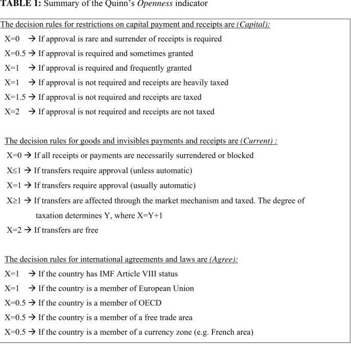
closed (0) to most open (12) economies. In addition, he uses a seventh dimension (Agree) which is a measure for the country’s participation in international legal agreements which constraints the country’s ability to restrict exchange and capital flows. In this dimension a country has a score of 0, .5, 1, 1.5, or 2 ranging from not constrained at all to very con-strained. The resulting composite 0-14 measure is called Openness (see Table 1 for further information).
TABLE 1: Summary of the Quinn’s Openness indicator
The decision rules for restrictions on capital payment and receipts are (Capital): X=0 Æ If approval is rare and surrender of receipts is required
X=0.5 Æ If approval is required and sometimes granted X=1 Æ If approval is required and frequently granted
X=1 Æ If approval is not required and receipts are heavily taxed X=1.5 Æ If approval is not required and receipts are taxed
X=2 Æ If approval is not required and receipts are not taxed
The decision rules for goods and invisibles payments and receipts are (Current) : X=0 Æ If all receipts or payments are necessarily surrendered or blocked X≤1 Æ If transfers require approval (unless automatic)
X=1 Æ If transfers require approval (usually automatic)
X≥1 Æ If transfers are affected through the market mechanism and taxed. The degree of taxation determines Y, where X=Y+1
X=2 Æ If transfers are free
The decision rules for international agreements and laws are (Agree): X=1 Æ If the country has IMF Article VIII status
X=1 Æ If the country is a member of European Union X=0.5 Æ If the country is a member of OECD
X=0.5 Æ If the country is a member of a free trade area
X=0.5 Æ If the country is a member of a currency zone (e.g. French area)
This table is based on the coding rules as illustrated in Quinn 1997 (Appendix A: Data on International Finan-cial Regulation, p. 544. Quinn (1997))
4.1.2 The IMF Dummy Measure
Besides the information about the exchange rate system and exchange rate restrictions for in-dividual country members the IMF’s Annual Report also includes a summary table “Summary Features of Exchange and Trade Systems in Member Countries” specifying whether given forms of exchange arrangements and restrictions are adopted by member countries since the 1967 issue (covering 1966). In this table IMF computes an indicator of presence or absence of restrictions on payment by residents of current and capital account obligations. This level in-dicator is used in most studies and takes a value of either 0 or 1, as a dummy variable in re-gression models. Alesina, Grilli and Mi lesi-Ferreti (1994), Leblang (1995), Rodrik (1998), Razin and Rose (1994) use this indicator.
The structure of this 1 or 0 measure is not appropriate for most cases, however, in indicating the level of financial openness. One of the shortcomings of this measure is that, presence or absence of regulation gives no information about the magnitude of a nation’s financial restric-tion on current or capital payments by residents. Thus this indicator cannot measure the economies which are not fully open or fully closed. A second drawback, Quinn (1997) men-tioned is that the table does not contain information about important aspects of financial openness, such as restrictions on nonresident transactions (e.g., inward foreign direct invest-ment).
The IMF indicator cannot measure any changes in regulation (which is the subject of time series analysis). Taking the first difference of the IMF indicator (coded as 0 or 1) gives a data set of zeros interspersed with a handful of ones and minus ones . The table does not have
enough capacity to capture governments’ liberalization process or regulation in respect to in-ternational financial transaction.
4.1.3 A Comparison of Two Measures
Edwards (2001) makes a comparison between these two indicators, namely, Quinn measure and the IMF dummy measure. He computes the latter for three periods (1981-1985, 1986-1990, 1981-1990) and for 61 countries. His summary statistics shows capital controls are more common among emerging countries. The results also show that during the second half of the 1980s, the emerging countries increased the controls while industrial countries reduced them. He then applies Kruskal-Wallis test to see if it is statistically different in emerging and industrial countries. Again, the test statistics indicated that capital controls turn out to be sig-nificantly larger in emerging countries. Edwards also points out the shortcomings of the dummy index and criticizes its characteristic of not allowing to measure the positions at the intervals but in the extremes, as being subject to no controls, or completely closing up capital mobility. His calculations countries show that between 1980 and 1985 only eight, and be-tween 1985 and 1990 only three countries had values other than 0 or 5 extremes among the sample size of 61 countries. He argues that this character of the IMF dummy index decreases its usefulness in empirical cross section analyses.
He also computes the Quinn index for two periods (1973 as the mid 1970s; and ; 1987 as the mid/late 1980s) and used a sample of 65 countries and concludes that industrial countries have greater capital mobility than the emerging countries.
According to Edwards, Quinn indicator is superior to the 0 or 1 measure since it gives more information about the degree of capital mobility. The 0-4 scale reflects the degree of the capi-tal openness; the countries with higher number means a higher degree of capicapi-tal mobility. One other superior characteristics of Quinn’s index is that it is suitable for research of capital ac-count liberalization, since it can give information on the changes over time, not only on a particular period in time.
4.2 “De Facto” Openness Measures
The other way of measuring openness, the de facto openness, is an actual measure of capital flows such as FDI, portfolio investment and debt flows. The advantage of this type of meas-urement is that we use data which is directly what the country is experiencing. This is an im-portant point because a gap between the legal openness level and the openness that is actually realized is not unusual.
When measuring the de facto openness most important problem is that the opening process can be to some extent related to the factors in the economy not only determined exogenously. This problem is endemic to the De facto openness measures because magnitude of the actual capital inflows are likely to be closely related with investment opportunities, political and economic environment of the country and etc. This problem is not as important as for de jure measures like it is for de facto measures.
5
.
THE RELATIONSHIP BETWEEN CAPITAL ACCOUNT
LIBERALIZATION AND ECONOMIC PERFORMANCE
It is a common belief among the supporters of capital liberalization that the capital will move from capital-rich to capital-poor economies thus will improve the efficiency of world resource allocation. They also think that capital mobility will provide a more efficient global allocation of investment and more efficient domestic policies and let economic agents benefit of risk diversification. One of their main arguments is that international capital mobility is an engine of growth. Capital flows relax constraints on resource mobilization, convey technological and organizational knowledge and catalyze institutional change; the capital inflows can help the countries smooth consumption and finance investments and the investments ease the techno-logical and managerial know-how [Eichengreen (2003)]. Supporters of this approach have argued that, by increasing the rewards for good policies and the penalties for bad policies, capital flows can promote more disciplined macroeconomic policies. [Grilli and Milesi-Ferretti (1995)]
The arguments in favor of capital mobility and flows to developing countries are based upon a neoclassical framework. In total there are five different arguments in favor of external finan-cial liberalization. First, at the aggregate level, capital movements from developed to develop-ing countries are said to improve the efficiency of world resource allocation (Mathieson & Rojas-Suarez,1994). Secondly, external financial liberalization can induce investment and growth by supplementing domestic savings. Expansion of aggregate income, in turn, can fur-ther raise domestic savings and investment, fur-thereby creating a cycle in which fur-there is sus-tained economic growth. Thirdly, financial liberalization can also promote dynamic efficiency in the financial sector through foreign competition. Fourthly, capital flows to developing
countries create an opportunity for residents to hold diversified asset portfolios at the interna-tional level. Fifthly, it may ease access to internainterna-tional financial markets and reduce borrow-ing costs.
On the other side, the proponents of capital controls argues that the cross border transaction of capital causes significant external and domestic volatility particularly in less advanced na-tions. Reducing capital controls leaves countries more vulnerable to bank runs and financial panics which causes reversals in capitals flows. Rodrik (1998) clearly exposes this view: “A finance minister whose priority is to keep foreign investors happy will be one who pays less attention to developmental goals. We would have to have blind faith in the efficiency and ra-tionality of international capital markets to believe that these two sets of priorities will regu-larly coincide.”
The answer to these critics of the supporters of capital account liberalization is that the liber-alization can be vulnerable to the countries with poor financial system and those do not have a solid macroeconomic framework.
Quinn (1997) explores the same issue by tracing the following question: “Is international fi-nancial liberalization robustly associated with long-run economic growth in the cross-section of countries?”. He suggests adding the variable of capital account deregulation as one of the determinants of long-run economic growth beside investment and initial level of income and concludes that capital account deregulation has a positive effect on economic growth. He ap-plies a multivariate regression analysis for 64 countries to see the relations between change in international financial regulation and measures of long-run economic growth, corporate taxa-tion, government expenditures and income inequality. His study is the first multivariate
ex-amination of the connection between change in international financial regulation and a variety of political-economic outcomes.
6. CAPITAL ACCOUNT LIBERALIZATION AND ECONOMIC
PERFORMANCE: THE CASE OF TURKEY (1987-2004)
In this section, the long-run and short-run relationships between the GDP per capita growth and two types of de-jure capital openness measure are examined. These measures are portfo-lio over GDP and FDI over GDP. Granger causality test is used for the short-run while the error correction model (ECM) is used to test the long-run relationships.
6.1 The Methodology
The long-run and short-run relationships between the GDP per capita growth and two types of de-facto capital openness measures are examined in the analysis. These measures are portfolio investments over GDP and foreign direct investments over GDP. Granger causality test is used for the short-run while the error correction model (ECM) is used to test the long-run relationships.
6.1.1 Granger Causality Test
The existence of a correlation between variable do not always indicate a causality between those variables. Granger test is one of the ways to check the pairwise causality between the variables of interest.This approach of causality testing examines whether one variable causes
the other to see how much the actual value of one variable explained by its past values and then to see whether adding lagged values of the other can improve the explanation.
In other words, we run bivariate regressions of the form:
t k k t k t k t t t k k t k t k t t u y y x x x x x y y y + + + + + = + + + + + = − − − − − − − − β β α α α ε β β α α α ... .... ... .... 1 1 1 1 0 1 1 1 1 0
for all possible pairs of (x,y) series in the group. We then check the Wald statistics for the joint hypothesis: 0 ... 2 1 =β = =βk = β
for each equation. The null hypothesis is that x does not Granger-cause y in the first regres-sion and that y does not Granger-cause x in the second regresregres-sion.
It is important to note that the statement "x Granger causes y" does not imply that y is the ef-fect or the result of x. Granger causality measures precedence and information content but does not by itself indicate causality in the more common use of the term.
6.1.2 Testing for The Unit Root
As most of the time-series economic data are non-stationary, in order to avoid spurious re-gressions, first of all we need to check whether the variables are stationary or not. We chose to perform the standard Augmented Dickey-Fuller Test (ADF). Before applying ADF -using the Akaike Information Criterion (AIC)- we determined the optimal lag length to avoid auto-correlation in the residuals and to provide a better fit for the ADF test. Only after all series examined are integrated of the same order, we can continue with testing for both the long and short-run relationships.
6.1.3 Engle-Granger Two- Step Procedure
One of the approaches to testing for co-integration is Engle-Granger Two-Step Procedure, so-called residual based test. The first step of the Engle-Granger two-step procedure is to apply OLS on the equation:
t t
t x
y =α+β +ε
The variables co-integrate if εˆ is integrated of order zero where t εˆ is the estimated residuals. t The second step is to employ Augmented Dickey-Fuller unit root test of the estimated residuals. The ADF model can be expressed as follows:
t t k i t t= + + Δ +z Δ − = −
∑
1 1 1 ˆ ˆ ˆα
π
ε
ε
ε
where is an error term. If the null hypothesis of
z
t π =0 is rejected, then it can be conluded that residuals are integrated of order zero and the variables are cointegrated. Since the estimated residuals come from an OLS model, ADF critical values cannot be used. Instead, the MacKinnon’s critical values are considered when the residudals are tested since they give more accurate results compared to ADF critical values.6.1.4 Single Error Correction Model
For the bivariate models, single error correction model can be used to determine whether a long run relationship exists or not. Once, the estimated residuals are found to be integrated of order zero through Engle-Granger two-step procedure, eerror terms from the OLS can be used as an error correction term in the model. Error correction model can be formulated as follows:
t t i t k i i t k i t y x u y = + Δ + Δ + + Δ − − = − =
∑
∑
1 0 2 1 1 0α
α
λ
ε
ˆα
where λ is the speed of adjustment parameter, is assumed to be . We conclude a long-run relationship exists if
t
u NID(0,σ2)
λ, the coefficient for the lagged values of the estimated re-siduals turns out to be significant. Since t-statistics of λis closer to the normal distribution, we are going to use t-probability value to test whether there is cointegration between two variables.
6.2 The Data
This study analyses the relation between Portfolio investments and GDP Growth in the short and in the long run and the relation between FDI and GDP Growth in the long and in the short run. Turkey is examined for 17 years from 1987 to 2004. Three variables used in the analysis.
6.2.1 FDI: Foreign Direct Investment (FDI) is calculated as a share of GDP. The data is taken from the World Development Indicators. Foreign direct investment are the net inflows of investment to acquire a lasting management interest (10 percent or more of voting stock) in an enterprise operating in an economy other than that of the investor. It is the sum of equity capital, reinvestment of earnings, other long-term capital, and short-term capital as shown in the balance of payments. This series shows net inflows in the reporting economy. Data are in current U.S. dollars. The source is International Monetary Fund, International Fi-nancial Statistics and Balance of Payments databases, and World Bank, Global Development Finance.
6.2.2 GDP Growth:Annual percentage growth rate of GDP at market prices based on constant local currency. Aggregates are based on constant 2000 U.S. dollars. GDP is the sum of gross value added by all resident producers in the economy plus any product taxes
and minus any subsidies not included in the value of the products. It is calculated without making deductions for depreciation of fabricated assets or for depletion and degradation of natural resources. The source is World Bank national accounts data, and OECD National Ac-counts data files.
6.2.3 Portfolio Investments: Portfolio bond investment consists of bond issues purchased by foreign investors. Data are in current U.S. dollars. The source is World Bank, Global Development Finance. (http://devdata.worldbank.org/dataonline/)
6.3 Effects of Portfolio Investments on The Economic Performance
6.3.1 Short Run Analysis
The prerequisite for running a Granger causality test is to ascertain that the variables are I(0). The Augmented Dickey-Fuller (ADF) test is conducted to test the unit root and thus to find out the level of the order of integration.
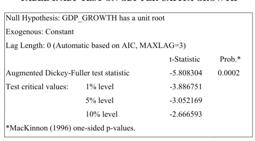
ADF test is first applied to the GDP per capita growth. The hypothesis is that GDP per capita growth has a unit root. ADF test result is significant meaning that the null hypothesis of GDP per capita growth has a unit root is rejected. (The ADF test statistics is greater in absolute value than the critical values according to the 1% and 5% confidence level.)
TABLE 1. ADF TEST ON GDP PER CAPITA GROWTH
Null Hypothesis: GDP_GROWTH has a unit root Exogenous: Constant
Lag Length: 0 (Automatic based on AIC, MAXLAG=3)
t-Statistic Prob.* Augmented Dickey-Fuller test statistic -5.808304 0.0002 Test critical values: 1% level -3.886751
5% level -3.052169
10% level -2.666593
*MacKinnon (1996) one-sided p-values.
The unit root test is also performed for the openness measure of portfolio over GDP. ADF test result is also significant for portfolio over GDP. The null hypothesis that portfolio over GDP has a unit root is rejected according to the 1% and 5% confidence level.
TABLE 2. ADF TEST ON PORTFOLIO/GDP Null Hypothesis: PORT_OVER_GDP has a unit root
Exogenous: Constant
Lag Length: 1 (Automatic based on AIC, MAXLAG=3)
t-Statistic Prob.* Augmented Dickey-Fuller test statistic -4.80579 0.0019 Test critical values: 1% level -3.92035
5% level -3.06559
10% level -2.67346
*MacKinnon (1996) one-sided p-values.
Thus we conclude that neither of the variables, portfolio and GDP a growth has unit root. Af-ter controlling for the unit roots of the variables, Engle-Granger causality test can be now conducted.
Optimal lag length is assumed to be 2. Our null hypothesis is that portfolio does not Granger cause GDP growth. The Granger causality test result suggests that portfolio over GDP does not cause GDP growth.
TABLE 3: GRANGER CAUSALITY TEST (2LAG)
Pairwise Granger Causality Tests Sample: 1987 2004
Lags: 2
Null Hypothesis: Obs F-Statistic Probability
PORT_OVER_GDP does not Granger Cause GDP_GROWTH 16 2.39766 0.1367 GDP_GROWTH does not Granger Cause PORT_OVER_GDP 4.25996 0.04266
If we assume 3 lags rather than 2 the results do not change, we still cannot conclude a relation between the variables.
TABLE 4: GRANGER CAUSALITY TEST (3LAG)
Pairwise Granger Causality Tests Sample: 1987 2004
Lags: 3
Null Hypothesis: Obs F-Statistic Probability
PORT_OVER_GDP does not Granger Cause GDP_GROWTH 15 1.540065 0.277546 GDP_GROWTH does not Granger Cause PORT_OVER_GDP 2.810699 0.107811
The residual graph of the regression of GDP growth on portfolio assists us to find out outlier points. According to the residual graph there are sharp deviations are recognizable at years 1994, 1999 and 2001. Hence, dummy variables for the periods of 1994, 1999 and 2001 can be introduced in the model. These deviations make sense since Turkish economy faced destruc-tive crises in those years.
TABLE 5: REGRESSION ANALYSIS OF PORTFOLIO INVESTMENT ON GDP GROWTH (OLS)
Dependent Variable:
GDP_GROWTH Method: Least Squares
Sample: 1987 2004 Included observations: 18
Variable Coefficient Std. Error t-Statistic Prob.
PORT_OVER_GDP 44.3509 136.5727 0.324742191 0.749583
C 1.736177 1.834341 0.946485787 0.357977
R-squared 0.006548 Mean dependent var 2.164656
Adjusted R-squared -0.05554 S.D. dependent var 5.262287 S.E. of regression 5.406454 Akaike info criterion 6.317503 Sum squared resid 467.6759 Schwarz criterion 6.416433
Log likelihood -54.8575 F-statistic 0.105457
Durbin-Watson stat 2.5212 Prob(F-statistic) 0.749583
GRAPH 1: THE RESIDUALS FROM OLS
-12 -8 -4 0 4 8 1988 1990 1992 1994 1996 1998 2000 2002 2004 GDP_GROWTH Residuals
After introducing the dummy variables into our two-lag model, the Granger Causality Test conducted with the 1994, 1999 and 2001 dummies. Hence our model becomes as follows (The minus signs in the parentheses stand for the number of years lagged):
GDP_GROWTH = C(1)*GDP_GROWTH(-1) + C(2)*GDP_GROWTH(-2) + C(3)*PORT_OVER_GDP(-1) + C(4)*PORT_OVER_GDP(-2) + C(5)*DUMMY_1994 + C(6)*DUMMY_1999+ C(7)*DUMMY_2001 + C(8)
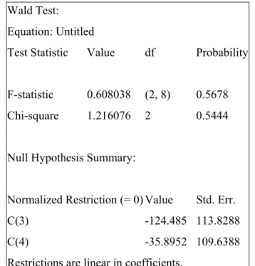
However, a statistically significant causality cannot be concluded. The short-run relationship between portfolio and GDP growth checked for all two year combinations: 1994 and 1999 dummies, 1999 and 2001 dummies, 1994 and 2001 dummies. We still could not conclude a significant causation. Then all the dummies are included one by one into the model. In this case, in the model where we used 1999 dummy alone, we concluded that portfolio investment causes GDP growth in the short run.
TABLE 6: GRANGER CAUSALITY TEST (2LAG) WITH DUMMY 94,99,2001
Wald Test: Equation: Untitled
Test Statistic Value df Probability
F-statistic 0.608038 (2, 8) 0.5678
Chi-square 1.216076 2 0.5444
Null Hypothesis Summary:
Normalized Restriction (= 0) Value Std. Err.
C(3) -124.485 113.8288
C(4) -35.8952 109.6388
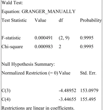
TABLE 7: GRANGER CAUSALITY TEST (2LAG) WITH DUMMY 94,2001
Wald Test:
Equation: GRANGER_MANUALLY
Test Statistic Value df Probability
F-statistic 0.000491 (2, 9) 0.9995
Chi-square 0.000983 2 0.9995
Null Hypothesis Summary:
Normalized Restriction (= 0) Value Std. Err.
C(3) -4.48952 153.0979
C(4) -3.44655 155.495
Restrictions are linear in coefficients.
TABLE 8: GRANGER CAUSALITY TEST (2LAG) WITH DUMMY 94,1999
Wald Test: Equation: Untitled
Test Statistic Value df Probability
F-statistic 4.252101 (2, 9) 0.0501
Chi-square 8.504202 2 0.0142
Null Hypothesis Summary:
Normalized Restriction (= 0) Value Std. Err.
C(3) -268.764 102.3734
C(4) -159.912 104.9844
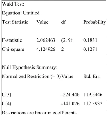
TABLE 8: GRANGER CAUSALITY TEST (2LAG) WITH DUMMY 1999, 2001
Wald Test: Equation: Untitled
Test Statistic Value df Probability
F-statistic 2.062463 (2, 9) 0.1831
Chi-square 4.124926 2 0.1271
Null Hypothesis Summary:
Normalized Restriction (= 0) Value Std. Err.
C(3) -224.446 119.5446
C(4) -141.076 112.5937
Restrictions are linear in coefficients.
TABLE 9: GRANGER CAUSALITY TEST (2LAG) WITH DUMMY 1994
Wald Test: Equation: Untitled
Test Statistic Value df Probability
F-statistic 1.39692 (2, 10) 0.2917
Chi-square 2.793841 2 0.2474
Null Hypothesis Summary:
Normalized Restriction (= 0) Value Std. Err.
C(3) -180.628 135.8075
C(4) -166.512 144.7062
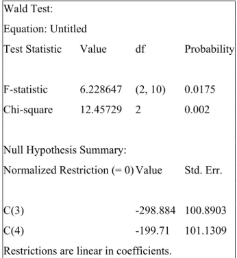
TABLE 10: GRANGER CAUSALITY TEST (2LAG) WITH DUMMY 1999
Wald Test: Equation: Untitled
Test Statistic Value df Probability
F-statistic 6.228647 (2, 10) 0.0175
Chi-square 12.45729 2 0.002
Null Hypothesis Summary:
Normalized Restriction (= 0) Value Std. Err.
C(3) -298.884 100.8903
C(4) -199.71 101.1309
Restrictions are linear in coefficients.
TABLE 11: GRANGER CAUSALITY TEST (2LAG) WITH DUMMY 2001
Wald Test: Equation: Untitled
Test Statistic Value df Probability
F-statistic 0.453683 (2, 10) 0.6477
Chi-square 0.907367 2 0.6353
Null Hypothesis Summary:
Normalized Restriction (= 0) Value Std. Err.
C(3) -106.744 145.3982
C(4) -112.843 145.6606
If all of the dummies were put in the model with three lags, Granger Causality Test gives a meaningful relationship between portfolio investment and GDP growth in the short-run.
TABLE 12: GRANGER CAUSALITY TEST (3LAG) WITH DUMMY 94,99,2001
Wald Test: Equation: Untitled
Test Statistic Value df Probability
F-statistic 14.50564 (3, 5) 0.0067
Chi-square 43.51693 3 0
Null Hypothesis Summary:
Normalized Restriction (= 0) Value Std. Err.
C(4) -195.373 84.49966
C(5) -65.0383 37.67801
C(6) -309.446 51.52784
Restrictions are linear in coefficients.
6.3.2 Long Run Analysis
In order to apply the ECM, we must check if the variables are cointegrated. In order to do this Engle-Granger two-step procedure is performed. The first step in this procedure is to regress GDP growth on portfolio investment. The second step is to check whether the residuals from this regression are I (0) or not. The existence of co integration is concluded if these residuals are I (0). However to run the regression mentioned in the first step, we have to check the unit roots of GDP growth and portfolio investment
Since we run the unit root test of Portfolio and GDP growth in the previous section, we know that these are I(0). The unit root test of the residuals must be run to ensure that every variable in our model have the same order of integration.
TABLE 13: ADF TEST ON RESIDUAL
Null Hypothesis: RESIDUAL_OLS has a unit root Exogenous: Constant
Lag Length: 0 (Automatic based on AIC, MAXLAG=3) t-Statistic Prob.* Augmented Dickey-Fuller test statistic -5.56073 0.000378 Test critical values: 1% level -3.88675
5% level -3.05217
10% level -2.66659
*MacKinnon (1996) one-sided p-values.
The null hypothesis is rejected in respect to 1% and 5% significance level concluding that the residual is also I (0). (ADF t-statistic is compared with MacKinnon’s critical value when ex-amining the unit root of residuals.)
It is now possible to apply error correction model in order to analyze the effect of portfolio on the GDP growth in the long run. The error correction model is formulated as follows:
t 1 t j t m 0 j i t k 1 i i 0 t
α
α
Δy
α
Δx
λ
εˆ
u
Δy
=
+
+
−+
−+
= − =∑
∑
jwhere λ is the speed of adjustment parameter, ut is assumed to be N (0, σ2)
The test results are insignificant meaning that there is no relation of Portfolio on the GDP growth in the long run.
TABLE 14: ERROR CORRECTION MODEL
Dependent Variable: D(GDP_GROWTH) Method: Least Squares
Sample (adjusted): 1990 2004
Included observations: 15 after adjustments
Variable Coefficient Std. Error t-Statistic Prob. D(GDP_GROWTH(-1)) 0.458427 0.656462 0.698329 0.5026 D(GDP_GROWTH(-2)) 0.211591 0.352917 0.599549 0.5636 D(PORT_OVER_GDP) 202.1616 137.378 1.471572 0.1752 D(PORT_OVER_GDP(-1)) 23.63341 133.8917 0.176511 0.8638 RESIDUAL_OLS(-1) -1.83527 0.846031 -2.16927 0.0582 C -0.29581 1.625007 -0.18204 0.8596
R-squared 0.736859 Mean dependent var 0.619387 Adjusted R-squared 0.590669 S.D. dependent var 9.133625 S.E. of regression 5.843598 Akaike info criterion 6.657745 Sum squared resid 307.3288 Schwarz criterion 6.940965 Log likelihood -43.9331 F-statistic 5.040434 Durbin-Watson stat 1.890401 Prob(F-statistic) 0.017708
When the 1994, 1999 and 2001 dummies are all added to the model the results change. In other words, if we control for the outlier financial crises years, the long run relation causality becomes significant. But this time the dummy variable of 1999 turns significant. So, the dummy variable of 1999 is excluded from the model. Afterwards, a new error correction model is constructed with 1994 and 2001 dummy variables. The t-probability result for this result is significant. Thus we conclude that there is a long run relation between portfolio investment and GDP growth.
TABLE 15: ERROR CORRECTION MODEL WITH DUMMIES FOR YEARS 1994, 1999 AND 2001
Dependent Variable: D(GDP_GROWTH) Method: Least Squares
Date: 07/27/06 Time: 17:14 Sample (adjusted): 1990 2004
Included observations: 15 after adjustments
Variable Coefficient Std. Error t-Statistic Prob.
D(GDP_GROWTH(-1)) 0.466634 0.464569 1.004445 0.3539 D(GDP_GROWTH(-2)) 0.269166 0.252766 1.064884 0.3279 D(PORT_OVER_GDP) -55.3136 160.8762 -0.34383 0.7427 D(PORT_OVER_GDP(-1)) 43.75858 72.70011 0.601905 0.5693 DUMMY_1994 -12.6344 3.964375 -3.18698 0.0189 DUMMY_1999 -6.92707 5.83323 -1.18752 0.2799 DUMMY_2001 -17.7416 7.172465 -2.47356 0.0482 RESIDUAL_OLS(-1) -1.78777 0.642493 -2.78255 0.0319 C 2.134712 0.845151 2.525833 0.0449
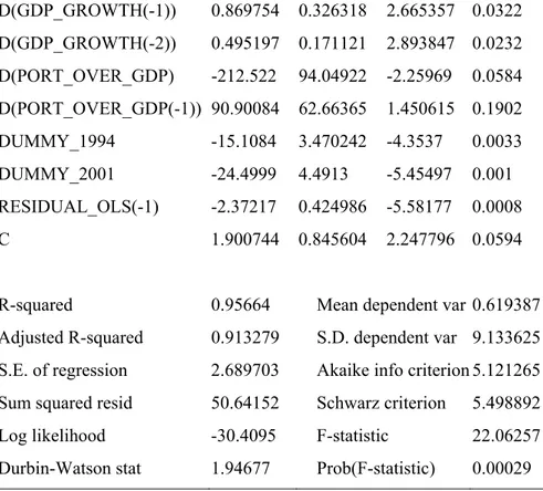
TABLE 16: ERROR CORRECTION MODEL WITH DUMMY 94 AND 2001
Dependent Variable: D(GDP_GROWTH) Method: Least Squares
Sample (adjusted): 1990 2004
Included observations: 15 after adjustments
Variable Coefficient Std. Error t-Statistic Prob.
D(GDP_GROWTH(-1)) 0.869754 0.326318 2.665357 0.0322 D(GDP_GROWTH(-2)) 0.495197 0.171121 2.893847 0.0232 D(PORT_OVER_GDP) -212.522 94.04922 -2.25969 0.0584 D(PORT_OVER_GDP(-1)) 90.90084 62.66365 1.450615 0.1902 DUMMY_1994 -15.1084 3.470242 -4.3537 0.0033 DUMMY_2001 -24.4999 4.4913 -5.45497 0.001 RESIDUAL_OLS(-1) -2.37217 0.424986 -5.58177 0.0008 C 1.900744 0.845604 2.247796 0.0594
R-squared 0.95664 Mean dependent var 0.619387 Adjusted R-squared 0.913279 S.D. dependent var 9.133625 S.E. of regression 2.689703 Akaike info criterion 5.121265 Sum squared resid 50.64152 Schwarz criterion 5.498892 Log likelihood -30.4095 F-statistic 22.06257 Durbin-Watson stat 1.94677 Prob(F-statistic) 0.00029
6.4 Effects of FDI on The Economic Performance
The other measure of openness, which is foreign direct investment over (FDI) over GDP, is taken into account in this section. The same procedure, followed in the previous section, is applied for the relationship between FDI and GDP growth. The ADF test is applied to the FDI and it is found that FDI does not have a unit root.
TABLE 17. AUGMENTED DICKEY-FULLER UNIT ROOT TEST ON FDI/GDP
Null Hypothesis: FDI_OVER_GDP has a unit root Exogenous: Constant
Lag Length: 0 (Automatic based on AIC, MAXLAG=3)
t-Statistic Prob.* Augmented Dickey-Fuller test
statis-tic -3.8185 0.0114
Test critical values: 1% level -3.88675
5% level -3.05217
10% level -2.66659
*MacKinnon (1996) one-sided p-values.
6.4.1 Short Run Analysis
The short run relationship between FDI and GDP growth is examined in this section. It is not possible to conclude a statistically significant causation using two lags. Therefore the Granger causality test applied for three lags. We still cannot reject the hypothesis that FDI does not Granger cause GDP growth.
TABLE 18: GRANGER CAUSALITY TEST (2LAG)
Pairwise Granger Causality Tests Sample: 1987 2004
Lags: 2
Null Hypothesis: Obs F-Statistic Probability
GDP_GROWTH does not Granger Cause FDI_OVER_GDP 16 1.252087 0.323658 FDI_OVER_GDP does not Granger Cause GDP_GROWTH 0.490748 0.624955
TABLE 19: GRANGER CAUSALITY TEST (3LAG)
Pairwise Granger Causality Tests Sample: 1987 2004
Lags: 3
Null Hypothesis: Obs F-Statistic Probability
FDI_OVER_GDP does not Granger Cause GDP_GROWTH 15 0.43479 0.73407 GDP_GROWTH does not Granger Cause FDI_OVER_GDP 1.5497 0.27535
In order to determine the outliers, OLS regression is conducted. The residual graph shows serious deviations in years 1994 and 1999. Hence, 1994 and 1999 dummies are added to the model.
TABLE 20: REGRESSION ANALYSIS OF PORTFOLIO INVESTMENT ON GDP_GROWTH (OLS)
Dependent Variable: GDP_GROWTH Method: Least Squares
Sample: 1987 2004 Included observations: 18
Variable Coefficient Std. Error t-Statistic Prob.
FDI_OVER_GDP -573.186 260.3791 -2.20135 0.0427
C 5.56732 1.908882 2.916535 0.0101
R-squared 0.232465 Mean dependent var 2.164656 Adjusted R-squared 0.184494 S.D. dependent var 5.262287 S.E. of regression 4.752128 Akaike info criterion 6.059501 Sum squared resid 361.3235 Schwarz criterion 6.158431 Log likelihood -52.5355 F-statistic 4.845955 Durbin-Watson stat 2.203069 Prob(F-statistic) 0.042734
GRAPH 2 : RESIDUAL OF OLS -12 -8 -4 0 4 8 1988 1990 1992 1994 1996 1998 2000 2002 2004 FDI_RESID
The Granger Causality Test employed for both two-lag and three-lag with 1994 and 1999 dummies.
TABLE 21: GRANGER CAUSALITY (2LAG) WITH DUMMY FOR THE YEARS 1994, AND 1999
Wald Test: Equation: Untitled
Test Statistic Value df Probability
F-statistic 0.802363 (2, 9) 0.4779
Chi-square 1.604727 2 0.4483
Null Hypothesis Summary:
Normalized Restriction (= 0) Value Std. Err.
C(3) 38.38454 320.7796
C(4) 389.8006 321.4446
TABLE 21: GRANGER CAUSALITY (3LAG) WITH DUMMY FOR THE YEARS 1994 AND 1999
Wald Test: Equation: Untitled
Test Statistic Value df Probability
F-statistic 0.556109 (3, 6) 0.6629
Chi-square 1.668328 3 0.644
Null Hypothesis Summary:
Normalized Restriction (= 0) Value Std. Err.
C(4) 147.3186 434.0638
C(5) 329.2472 346.9162
C(6) 222.2327 363.473
Restrictions are linear in coefficients.
The hypothesis that the coefficients of the FDI are simultaneously zero, cannot be rejected in both cases. Hence, we cannot conclude a short run relation between FDI and GDP growth.
6.4.2 Long Run Analysis
ECM model is conducted in this section. Before starting to use the ECM model, we must first show that the variables are cointegrated. For this purpose, Engle-Granger two step procedure is used to see whether the residuals are stationary or not.
TABLE 22: ADF TEST ON RESIDUAL Null Hypothesis: FDI_RESID has a unit root Exogenous: Constant
Lag Length: 0 (Automatic based on AIC, MAXLAG=3)
t-Statistic Prob.*
Augmented Dickey-Fuller test statistic -4.45581 0.0033 Test critical values: 1% level -3.88675
5% level -3.05217
10% level -2.66659
*MacKinnon (1996) one-sided p-values.
The hypothesis is tested by comparing ADF test value with the MacKinnon’s critical value. The null hypothesis that the residuals have a unit root is rejected because the ADF t-value is lower than the MacKinnon’s critical value at 5% and 1% significance level.
ECM can be now performed. It can be clearly seen from the output table of the ECM that there is a significant relationship between the FDI and GDP growth in the long run.
TABLE 23: ERROR CORRECTION MODEL
Dependent Variable: D(GDP_GROWTH) Method: Least Squares
Sample (adjusted): 1990 2004
Included observations: 15 after adjustments
Variable Coefficient Std. Error t-Statistic Prob. D(GDP_GROWTH(-1)) 0.399169 0.572512 0.697224 0.503273 D(GDP_GROWTH(-2)) 0.236511 0.33286 0.710542 0.495367 D(FDI_OVER_GDP) -557.472 264.7679 -2.10551 0.064538 D(FDI_OVER_GDP(-1)) -359.553 313.1726 -1.1481 0.280528 RESIDUAL_OLS(-1) -1.80762 0.790515 -2.28664 0.048038 C -0.20741 1.455038 -0.14254 0.88979
R-squared 0.786367 Mean dependent var 0.619387 Adjusted R-squared 0.667682 S.D. dependent var 9.133625 S.E. of regression 5.265261 Akaike info criterion 6.449313 Sum squared resid 249.5068 Schwarz criterion 6.732533 Log likelihood -42.3698 F-statistic 6.625672 Durbin-Watson stat 2.117835 Prob(F-statistic) 0.007472
7. CONCLUSION
This study examines the long-run and the short-run relationships between the GDP per capita growth and two types of de-facto capital openness measures: portfolio investments/GDP and FDI/GDP. The advantage of this type of an openness measurement, compared to the de-jure measures such as Quinn and IMF dummy, is that we use the data which is directly what the country is experiencing.
Granger causality test is used to examine the short-run relationship while the error correction model (ECM) is used for the long-run analysis. These analyses showed that the short run rela-tion between FDI and GDP growth does not exist even if we introduced several dummy vari-ables. Beside that the short run causality test for portfolio investment concluded that higher portfolio investment leads to higher economic growth in the short run. However, this was pos-sible only when we introduced a dummy variable for the outlier year 1999. The long run cau-sality relation between portfolio investment and economic growth turned out to be significant when we add dummy variables for the two years of economic crises: 1994 and 2001 (The dummy variable of the other outlier year, 1999, was not significant, therefore we excluded this variable from our model). A long run relation between FDI and GDP growth is found in our model without introducing any dummy.
To conclude, our time-series case study results support the idea that FDI and portfolio invest-ments are driving forces for growth in the long run and portfolio investment enhances the economic growth also in the short run.
REFERENCES
Anderson, J. 2003. “Capital Account Controls and Liberalization: Lessons for India and China.” UBS Investment Research Report.
Barro, Robert J. 1991. “Economic Growth in a Cross-Section of Countries” Quarterly Journal of Economics 106: 407-43.
Brune, N. and Guisinger Alexandra. 2003. “The Diffusion Of Capital Account Liberalization in Developing Countries.” American Political Science Association, August.
Creane, Susan; Goyal, Rishi; Mobarak, A. Mushfiq and Sab, Randa. 2003. “Financial Devel-opment and Economic Growth in the Middle East and North Africa.” Newsletter of the Eco-nomic Research Forum, for the Arab Countries, Iran & Turkey, Volume 10: Number 2.
Dooley, Michael P. 1995. “A Survey of Academic Literature on Controls over International Capital Transactions.” NBER Working paper series, Working Paper 5352.
Edison, J. Hali; Klein, Michael; Ricci, Luca and Slok, Torsten. 2002. “Capital Account Liber-alization and Economic Performance: Survey and Synthesis.” IMF Working Paper.
Edwards S. 1998. “Barking Up the Wrong Tree.” Financial Times, October.
Edwards S. 1997. “Openness, Productivity and Growth: What Do We Really Know?.” Na-tional Bureau of Economic Research, Working Paper, March, No:5978.
Edwards S. 2001. “Capital Mobility and Economic Performance: Are Emerging Economies Different?” National Bureau of Economic, Research Working Paper No:8076.
Eichengreen Barry J. 2003. “Capital Flows and Crises.” MIT Press, Massachusetts.
Esen, Oğuz. 2000. “Financial Openness in Turkey.” International Review of Applied Econom-ics, Vol. 14, No. 1.
Grilli, V. and Gian, Maria Milesi-Ferretti. 1995. “Economic Effects and Structural Determi-nants of Capital Controls.” IMF Working Paper, March.
Ito, Hiro. 2004. “Is Financial Openness a Bad Thing? An Analysis on the Correlation Be-tween Financial Liberalization and the Output Performance of Crisis - Hit Economies.” Santa Cruz Center for International Economics, Paper 04-23.
Kim, Woochan. 2003. “Does Capital Account Liberalization Discipline Budget Deficit?” Re-view of International Economics, 11(5), 830–844.
Kraay, A. 1998. “In Search of the Macroeconomic Effects of Capital Account Liberalization.” The World Bank Group, October.
Leamer, E. 1983. “Let’s Take the Con Out of Econometrics.” American Economic Review, 73, 31-43
Leiderman, Leonardo and Razin, Assaf. 1994. “Capital Mobility: The Impact on Consump-tion, Investment and Growth.” Cambridge University Press.
Levine, R. and David, Renelt. 1992. “A Sensitivity Analysis of Cross-Country Growth Re-gressions.” The American Economic Review, 82(4), 942-963.
Narayan, Paresh Kumar and Smyth, Russell. 2004. “Temporal Causality and the Dynamics of Exports, Human Capital and Real Income in China.” International Journal of Applied Eco-nomics, Volume.1. 24-45.
Quinn D. 1997. “The Correlates of Change in International Financial Regulation.” The Ameri-can Political Science Review, Vol.91, No.3, 531-551.
Quinn, Dennis P. and Inclan, Carla. 1997. “The Origins of Financial Openness: A Study of Current and Capital Account Liberalization.” American Journal of Political Science, Vol. 41, No.3, 771-813.
Rodrik, D. 1998, “Who Needs Capital-Account Convertibility?” Essay in International Fi-nance No 207, Princeton University.
Stiglitz, Joseph A. 2000. “Capital Market Liberalization, Economic Growth, and Instability.” World Development 28, June: 1075-1086.
The MIT Dictionary of Modern Economics, Fourth Edition, Edited by David W. Pearce, The MIT Press Cambridge, Massachusetts, Sixth Printing, 1999.
White, H. 2001. Asymptotic Theory for Econometricians. Academic Press, New York.
Fratzscher, Marcel and Bussiere, Matthieu. 2004. “Financial Openness And Growth: Short-Run Gain, Long-Short-Run Pain?” ECB Working Paper Series, No.348