978-1-7281-1862-8/19/$31.00 ©2019 IEEE
Diffused Label Propagation based Transductive
Classification Algorithm for Word Sense
Disambiguation
Gökhan Kocaman Computer Engineering Department
Marmara University İstanbul, Turkey [email protected]
Bilge Şipal
Mathematics and Computer Science Department
İstanbul Kültür University İstanbul, Turkey [email protected]
Aydın Gerek
Computer Engineering Department Marmara University
İstanbul, Turkey [email protected] Berna Altınel
Computer Engineering Department Marmara University
İstanbul, Turkey [email protected]
Murat Can Ganiz Computer Engineering Department
Marmara University İstanbul, Turkey murat.ganiz @marmara.edu.tr
Abstract- A major natural language processing problem, word sense disambiguation is the task of identifying the correct sense of a polysemous word based on its context. In terms of machine learning, this can be considered as a supervised classification problem. A better alternative can be the use of semi-supervised classifiers since labeled data is usually scarce yet we can access large quantities of unlabeled textual data. We propose an improvement to Label Propagation which is a well-known transductive classification algorithm for word sense disambiguation. Our approach make use of a semantic diffusion kernel. We name this new algorithm as diffused label propagation algorithm (DILP). We evaluate our proposed algorithm with experiments utilizing various sizes of training sets of disambiguated corpora. With these experiments we try to answer the following questions: 1. Does our algorithm with semantic kernel formulation yield higherclassification performance than the popular kernels? 2. Under which conditions does a kernel design perform better than others? 3. What kind of regularization methods result with better performance? Our experiments demonstrate that our approach can outperform baseline in terms of accuracy in several conditions.
Keywords—natural language processing, word sense disambiguation, machine learning, transductive inference, label propagation, semantic diffusion kernel
I. INTRODUCTION
In every language there are some words which have more than one meaning. For example, the noun nail represents a part on our fingers and toes which is called fingernail and toenail, more specifically. Moreover, nails represent thin, sharp metal pieces used in construction. Another example of a word with more than one meaning is jam. One possible sense of the word jam could be a sweet paste made out of fruit. When used as a verb jam means to put something into a space that is too small for it. Another meaning of the word jam is when the cars on the road are very slow or stopped, which is called a traffic jam.
Humans subconsciously understand the right meaning easily by observing the context. On the other hand to computationally identify the suitable sense of the word is not a trivial task. Word sense disambiguation (WSD) is the problem of automatically finding which sense is the correct sense of a given word according to its context [1].
WSD is a very popular task in both academic and non-academic platforms. There is an extensive bibliography for resolving ambiguity of polysemous words. There are two variants of WSD tasks [2], lexical-sample task and all-words task. The main difference between lexical-sample task and all-words task is that the latter attempts to disambiguate all types of words (i.e., nouns, adjectives, verbs, adverbs…etc.) in the entire corpus while lexical-sample task deals with only pre-selected types of target words.
In order to resolve ambiguity several algorithms have been developed. It Makes Sense (IMS) is a supervised English all-words WSD system. Zhi and Ng [3] attempt to handle the WSD task with the IMS framework using the support vector machine (SVM) classifier and integrating multiple features such as part-of-speech (POS), surrounding words and local collocations. Taghipour and Ng [4] aim to incorporate word embeddings in a continuous space [5] to IMS framework in a WSD system. Iacobacci et al. [6], also use IMS framework and word embeddings as features and report that significant performance improvements are achieved. Melamud et al. [7] use context2vec with bidirectional long short-term memory (Bi-LSTM) to train word vectors. According to the experimental results, they get better results on the WSD task. Other efforts including LSTM and bi-LSTM are [8, 9, 10]. For instance the methodology in [8] has three layers; the softmax layer, a hidden layer and a Bi-LSTM layer. Bi-LSTM and hidden layer share parameters over all word types and senses. The output of the model is the concatenation of the outputs of left pass vector and right pass vector of LSTM. There is another model called gloss augmented WSD neural network (GAS) is introduced by [11].
We consider the WSD as a transductive classification problem and propose an improvement to Label Propagation which is a well-known transductive inference algorithm. Our approach make use of a semantic diffusion kernel. We name this new algorithm as diffused label propagation algorithm (DILP). We evaluate our proposed algorithm with experiments utilizing various sizes of training sets of disambiguated corpora accompanied with unlabeled data. With these experiments we try to answer the following questions: 1. Does our algorithm with semantic kernel formulation yield higherclassification performance than the popular kernels? 2. Under which conditions does a kernel design perform better than others? 3. What kind of regularization methods result in better performance? Our experiments demonstrate that our approach can outperform
baseline methods in terms of accuracy under we describe below.
II. BACKGROUND A. Word sense disambiguation
Word Sense Disambiguation (WSD) actually is a classification problem since it attempts to find the most suitable sense of a word among its possible senses defined by a dictionary based on its context. There are two variants of WSD tasks [2]. One is the Lexical sample task. In the Lexical sample task, there are only a small number of pre-selected types of target words. There is an inventory of senses of each word. Supervised machine learning approaches are used to train a classifier for each word. The second type of WSD task is the All-words task. The main difference between lexical sample task and all-words-task is that the All-words task attempts to disambiguate all types of words (i.e., nouns, adjectives, verbs, adverbs…etc.) in the entire corpus. This task generally needs wide-coverage systems [2].
B. Label Propagation Algorithm
Label Propagation (LP) [12] is a graph based semi-supervised transductive learning method. That means learning is limited to the given data. There are inductive methods which aims to model the whole sample space [13, 14].
There are two main assumptions behind the LP algorithm. First, closer data points tend to have similar class labels, which is the main logic behind K-Nearest Neighbor (KNN). Second, points on the same cluster are likely to have the same label [15]. The first assumption is a local assumption whereas the second is a global one. These two assumptions together are called the cluster assumption [16, 17].
The algorithm propagates the class label of a node in a graph to neighboring nodes by using weighted edges and proximity. This process is repeated until convergence to a unique solution is achieved, which is guaranteed [12]. Thus, the labeled data is used in a classification model to assign labels to the unlabeled data.
In this study, we employed the well-known LP algorithm [12], which is implemented in the Scikit-Learn Library1. Let
us explain the problem setup and the steps of the algorithm.
1https://scikit-learn.org/stable/#
For 𝑙, 𝑢 ∈ ℕ with 𝑙 < 𝑢 and 𝑙 + 𝑢 = 𝑛 we let 𝑋 = {𝑥 … 𝑥 } denote the array of contexts (documents) and each 𝑥 is a vector of dimension 𝑡 where 𝑡 denotes the number of terms. Hence X is a 𝑡𝑒𝑟𝑚 × 𝑑𝑜𝑐𝑢𝑚𝑒𝑛𝑡 matrix. We let class labels to denote senses of words to be disambiguated where 𝑌 = {𝑦 … 𝑦 } denotes the known senses (class labels), 𝑌 = {𝑦 … 𝑦 } denotes the unknown senses and 𝑌 = 𝑌 ∪ 𝑌 .
First, we form a fully connected graph whose vertices are (𝑥 , 𝑦 ) … (𝑥 , 𝑦 ). The edges between the vertices, say 𝑖, 𝑗 are weighted by using similarity score between the vectors 𝑥 and 𝑥, which is denoted by 𝑤 . The simplest
similarity score is the dot product of the vectors. Another popular way of computing the similarity is the radial basis function.
𝑤𝑖𝑗= 𝑒− ||𝑥𝑖−𝑥𝑗||2
2𝜎2 It results in larger weights when the distance between two vectors is closer. Radial Basis Function (RBF) is commonly used among other graph-based methods [12, 15, 18, 19].
The sigma parameter controls the weights. During the testing phase of this work we observed that the change in 𝜎 effects the model substantially, this is a well-observed phenomenon [17].
The LP model learns in two steps. In the first step, we use the similarity scores of the vectors in order to assign weights between nodes. Then we form the diagonal degree matrix, D as follows.
𝐷 = ∑ 𝑊
Bengio et al. claim that the algorithm works better if the diagonal elements of W are set to zero [20]. In the second part, the labels (senses in our case) are propagated until convergence. The initialization of 𝑌 is not important but for 𝑌 , we used two senses as labels. We choose the initialization of Y as 𝑌 = {𝑦 … 𝑦 , 0, … ,0} . After the initialization, the algorithm is as follows.
Fig. 1. Label Propagation Algorithm
Algorithm 1 returns the propagated labels which are then used to label the points in X. The matrix 𝑌 can be constructed differently when there are more than two classes as in [21]. For WSD, Niu et. al. 2005 used a 𝑑𝑜𝑐𝑢𝑚𝑒𝑛𝑡 × 𝑐𝑙𝑎𝑠𝑠 matrix with 𝑌 = 1 if 𝑦 is in sense tag 𝑠 and 𝑌 = 0 otherwise. Then they use the same algorithm in a one-versus-rest fashion.
Some other graph-based learning methods that are well-known are as follows: [19] is based on Markov random walks, [22] iteratively computes the distributions of labels (MAD algorithm), [23] is similar to Markov random walks,
[17] computes local structure and combines them to get a better global learner.
They generally have similar graph constructions but different regularizing methods or loss function. For an extensive survey on the topic one can refer to [20] or [24]. There are exceptions that focus on graph connectivity, for example, [1] studies extensively the structure of a given graph for unsupervised learning, but they are beyond the scope of his work.
III. RELATED WORK A. Approaches for WSD
There are several types of algorithms developed for WSD in the literature.
The IMS Framework: It Makes Sense (IMS) is a supervised English all-words WSD system. Zhi and Ng [3] present the IMS framework with the default support vector machine (SVM) classifier. Moreover, they integrate multiple features such as part-of-speech (POS), surrounding words and local collocations. It is a flexible framework which allows users to choose different features, classifiers and preprocessing tools. IMS+emb: Taghipour and Ng [4] aim to incorporate word
embeddings which are representations of words in a continuous space [5] in a WSD system. In their work they choose to work with the word embedding that is created by Collobert and Weston [26] which they name as CW. To produce a word representation using CW embedding, they use a feed forward neural network with stochastic gradient descent as the training algorithm. The WSD framework in use is IMS and they also construct the default settings of IMS as baseline. The idea behind using word embeddings in the WSD task is to add the distribution of the representation of the words to the system which leads the classifier to take the similarity of the words into account.
One other IMS based WSD method is Iacobacci et al. [6], who show that by designing IMS properly and employing word embeddings as features gives significant performance improvements which are hard to beat [11].
context2vec: Melamud et al. [7] introduce a different word embedding which they call context2vec. Their basic idea is to use bidirectional LSTM (Bi-LSTM) to train a word vector. Their model is based on word2vec's CBOW architecture [5] but they use Bi-LSTM instead of averaged word embeddings (AWE). They outperform AWE and they get similar or better results on WSD task (and some other tasks such as sentence completion and lexical substitution).
LSTM and Bi-LSTM: Long Short-Term Memory (LSTM) is a type of gated recurrent neural network [27] which is introduced for sequence models to make use of the long term dependencies, i.e. it preserves information from the preceding inputs(past). The bidirectional LSTM (Bi-LSTM) [28] is an adaptation of the LSTM which runs inputs both from the past and the future. As humans understand the sense of a word by observing the context, this WSD technique uses information about both preceding and succeeding words [8]. Their model has three layers; the softmax layer, a hidden layer and a Bi-LSTM layer. Bi-LSTM and hidden layer share parameters over all word types and senses. The output of the model is the concatenations of the outputs of left pass vector
and right pass vector of LSTM. Furthermore, there is an embedding layer that provides out the word embedding, which is GloVe [5] in their case. In order to decrease the dependency on individual word in the training set, they use the regularization technique [29]. Compared to IMS+adapted
CW and other naive Bi-LSTM methods, their model achieves state-of-the-art level improvements. One of the most important advantages of this model is that it is independent of the chosen language.
The model gloss augmented WSD neural network (GAS) is introduced by Luo et al. [11]. The main differences between this model and the Bi-LSTM model of [8] are the gloss module and the memory module of GAS. The gloss module makes use of the glosses (sense definitions) which is ignored by previous neural network models. This module can be seen as an embedding module of glosses which is trained by a Bi-LSTM. The aim of the memory module is to model the relationship between the glosses and the context. Experiments show that their model outperforms Raganata et al. [9], Kägeback and Salomonsson [8] and Iacobacci et al. [6].
B. Label Propagation Algorithms
Generally, in graph based learning algorithms, the graph constructions are similar [24] as we mentioned before. If we consider the given graph method as estimating a classification function 𝑓 , then the graph based algorithms differ by their loss function (how close 𝑓 estimates labels to the given ones) or regularizers (how smooth is 𝑓 on the whole graph).
For example, the methods with combinatorial graph Laplacian ℒ, are MinCuts [23], label propagation [12], and Gaussian random fields [12, 18]. The method that employs usage of kernels on graphs is manifold regularization [13]. Discrete regularization [15] uses normalized graph Laplacian. Interpolated and Tikhonov regularization employ 𝐿 regularization [14].
In our work we also focus on regularization of our graph based method by using a Kernel and a regularization method based of graph Laplacian. Before explaining graph Laplacian, let us discuss why such regularization is needed. As mentioned in several studies [13, 14, 15, 24], the classifier learned by the graph-based method has to be consistent with both the initial labeling and the geometry of the data. Rapid changes between close points cause the model to fail to fulfill the cluster assumption and it has to be punished for that.
One common way is to normalize the graph Laplacian as given in [15]. We add a regularization step in the initialization.
Then we iterate the following equation in the label propagation algorithm where 𝑌 is the initialization and t denotes the iteration steps [12].
𝑌𝑡+1← 𝛼ℒ𝑌𝑡+ (1 − 𝛼)𝑌
This new regularized algorithm is called label spreading [15, 20]. For a proof of the convergence of this algorithm, one can refer to [15]. Note that the eigenvalues of 𝛼ℒ are in (−1,1).
Another method that we mention here is the Kernel method. Kernels among nodes are referred to as kernels on graphs and it should not be mixed with graph kernels [30]. The most popular kernel used for label propagation is the radial basis kernel or Gaussian kernel,
𝐾(𝑥, 𝑥 ) = exp || || where 𝜎 is the scaling parameter. By some parameters change, it is the solution of the diffusion equation (Kondor et. al. 2004). In physics, the diffusion equation describes how heat and gas diffuse in homogenous environment with time. Intuitively, in graph based learning methods, we want the given labels to diffuse over the whole graph. This intuition explains why Gaussian kernels are very popular in graph based learning methods. For a formal proof, one can refer to [13, 15, 31]. The heat or gas equations are all in a continuous setting, but our problem is a discrete one. In [31, 32] a discretization of a Gaussian kernel by using the graph Laplacian is introduced that is called the diffusion kernel
𝐾𝜆 = 𝑒𝑥𝑝(𝜆ℒ) = 𝑙𝑖𝑚 → (𝐼 + ℒ ) = 𝐼 + 𝜆ℒ + ℒ + ⋯
where ℒ is the graph Laplacian of the graph and 𝜆 is control parameter. Note that, the powers of positive semi definite matrices are positive semi-definite and this way positive definiteness is assured.
Semantic Diffusion Kernel: This idea of using the diffusion kernel in a discrete setting such as text classification and particularly in word sense disambiguation is not new. Very recently, Wang et al. [25] proposed a semantic diffusion kernel which uses semantic similarities as a diffusion process in a graph whose nodes represent the contexts and edges represent the first-order similarities.
Diffusion considers all possible paths connecting two nodes in the graph. The basic idea of the algorithm is to construct an augmented term-document matrix. Then by applying the "Diffusion" process to this matrix so that the words which are in the same class become closer to each other.
In [25, 33] they used this technique with support vector machines to capture the higher order correlations between terms. Let us explain how they created their diffusion matrix in detail. First, they get a 𝑡𝑒𝑟𝑚 × 𝑡𝑒𝑟𝑚 matrix 𝐺 = 𝑋 𝑋 and compute the following.
𝑆 = exp 𝐺 = 2𝐼 + 𝜆𝐺 +
! + ⋯ (6)
The matrix 𝑆 is called a semantic similarity matrix. Then they compute 𝑑𝑜𝑐𝑢𝑚𝑒𝑛𝑡 × 𝑑𝑜𝑐𝑢𝑚𝑒𝑛𝑡 semantic diffusion kernel 𝐾 = 𝑋 𝑆 𝑆𝑋, which they used for SVM. According to their experiments their diffusion kernel is superior to LSI and linear kernel with several SensEval disambiguation tasks such as interest, line, hard and serve. The Diffusion algorithm is shown in the following Figure.
Fig. 2. Diffusion Kernel Algorithm
Other semi-supervised WSD studies with LP are [21] that uses label propagation with similarities (cosine, Jensen-Shannon divergence) and get very good results, [34], which uses basic dot product with LP, on parallel corpora and applies on Chinese data sets. Recent works generally focus more on merging label propagation method with deep learning methods such as LSTM [35]. As far as we know, none of them used semantic diffusion kernels in their work. IV. APPROACH
In our work, we apply label propagation for the WSD task. The Laplacian regularization method is employed to keep the local global consistency. Then we used the DILP instead of RBF kernel to capture the semantic similarities and to get a smooth decision surface. Finally, we compared our results with the RBF kernel. According to the experimental results on WSD task, DILP gives higher classification accuracy in compare to RBF. Following figure shows the detail about DILP.
Fig. 3. Diffused Label Propagation (DILP) Algorithm V. EXPERIMENTS AND RESULTS A. Datasets
In order to evaluate our algorithm we select the datasets namely hard, line, serve and interest from SensEval. This dataset is used in the studies of WSD. Word occurences in all dataset were manually tagged with a WordNet sense.
Hard Data: There are 4333 instances in hard data. These instances are labeled as HARD1, HARD2 and HARD3.
Line Data: The line data contains 4146 instances. Six different senses and frequencies are shown on Table 1.
Serve Data: 4378 instances occur in this dataset. Moreover Table 1 shows four different senses and their frequencies.
Interest Data: It has 2367 instances. There are six senses in this dataset and their details are shown on Table 1.
TABLE I. DATASETS
Name No Sense Frequency
Hard
1 not easy (difficult) 3455
2 not soft (metaphoric) 502
3 not soft (physical) 376
Line
1 Stand in line 349
2 A nylon line 373
3 A line between good and evil 374
4 A line from Shakespeare 404
5 The line went dead 429
6 A new line of workstations 2217
Serve
1 Function as something 853
2 Provide a service 439
3 Supply with food 1814
4 Hold an office 1272
Interest
1 Readiness to give attention 361 2 Quality of causing attention to be given 11 3 Activity, etc. That one gives attention to 66 4 Advantage, advancement or favor 177 5 A share in a company or business 500 6 Money paid for the use of money 1252 B. Experimental Setup
In order to observe the behavior of our approach under different training set size conditions we vary the labeled data percentage and report 40%, 50% and 60% where the performance difference of DILP is most visible. During experiments we optimized the parameters of DILP. For instance as similarity metric we use dot product and cosine similarity, and we choose dot product since it performs better.
For DILP there are three main parts, calculation the affinity matrix for dot product, normalization the graph Laplacian and Taylor expansion. We make some combinations for these three calculations and get crucial results. For example we use dot product with normalization, dot product with Taylor expansion, only Taylor expansion, only normalization etc.
Our approach works best in the binary classification scenario. Therefore, for each dataset we select two of the largest senses (classes) whose sizes are similar. For interest dataset we chose senses 1 and 5, that are the second and third largest classes. For line dataset we choose senses 4 and 5, again second and third largest senses with similar number of instances. Using a similar approach, we select senses 2 and 3 for Hard dataset, and senses 2 and 6 for Serve dataset for our binary classification experiments.
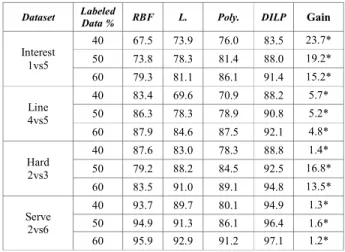
C. Evaluation Results and Discussions
Table II. represents the accuracy of each kernel for different training ratio of datasets. For each dataset we run experiments for 40, 50, and 60 training ratio. Our aim is presenting the higher accuracy of DILP opposed to other algorithms especially RBF. RBF is the baseline algorithm because for label propagation it gives the highest accuracy.
Especially this accuracy can be seen in scikit learn framework with optimized parameters. For interest data we can infer that 40% training data DILP gives the highest results. For 50% training data the result of RBF is 73.8% and DILP’s result is 88.0%. But on the below row which has 50% training data, the result of DILP rises to 91.4% and the closest one is 86.1% .Other datasets, line, hard and serve also give the similar results. On serve data the results of RBF and DILP are very closed but the highest score still remains the same algorithm which is DILP. However, performance gain between baseline algorithm and DILP is calculated as:
GainDILP = (PDILP – Px) / Px (7)
where PDILP is the classification accuracy of DILP and Px
represents the classification accuracy of RBF. Experimental results are also shown in Table II. The gain column which is the last column in Table II, demonstrates the (%) of DILP over RBF computed as in Eq. (7).
As a result, DILP became more successful than RBF (baseline kernel) with high labeled ratio such as on below table. On the other hand linear and polynomial kernels can exceed the RBF but not the DILP. Table II shows the results of RBF, linear, polynomial and DILP kernels on serve data with different size of training data. Furthermore, it shows that DILP gives the best result. In the below table L. represents linear kernel, and Poly. shows the polynomial kernel. The last column Gain is the percentage gain of DILP over RBF. Moreover the stars near gain values show the positive gain of DILP over RBF. In the training sets, where DILP significantly differs over RBF kernel based on Students t-Tests, we indicate this with “*”.
TABLE II. CLASSIFICATION ACCURACY RESULTS ON INTEREST,LINE,
HARD AND SERVE DATASETS
Dataset Labeled Data % RBF L. Poly. DILP Gain
Interest 1vs5 40 67.5 73.9 76.0 83.5 23.7* 50 73.8 78.3 81.4 88.0 19.2* 60 79.3 81.1 86.1 91.4 15.2* Line 4vs5 40 83.4 69.6 70.9 88.2 5.7* 50 86.3 78.3 78.9 90.8 5.2* 60 87.9 84.6 87.5 92.1 4.8* Hard 2vs3 40 87.6 83.0 78.3 88.8 1.4* 50 79.2 88.2 84.5 92.5 16.8* 60 83.5 91.0 89.1 94.8 13.5* Serve 2vs6 40 93.7 89.7 80.1 94.9 1.3* 50 94.9 91.3 86.1 96.4 1.6* 60 95.9 92.9 91.2 97.1 1.2*
VI. CONCLUSIONS AND FUTURE DIRECTIONS
Experimental results show that our approach, the DILP algorithm performs considerably better than the baselines RBF, linear and polynomial in labeled data percentages of %40, %50 and %60 in binary classification scenario. One of the conclusions driven from this study is that dot similarity affects the score better than the cosine similarity. Another affect is about the Taylor step. Detecting the most efficient
step has a crucial role on getting high score. The gamma value optimization also helps the score getting higher. One of the most effective optimization is using normalization with Taylor expansion. So these above optimization parameters make DILP, gives the best result in compare to RBF, linear and polynomial kernel.
As a future work, we extend DILP algorithm to perform multi-class classification using an appropriate method such as one versus all or one versus one approaches. Additionally, we aim to perform more experiments on other larger scale WSD corpora. We will also analyze how the other regularization methodologies with DILP improve classification accuracy in WSD in some test cases. An additional item in our agenda is to expand our approaches by adding further semantic-information and investigate how the construction of the used graph can affect the performance.
ACKNOWLEDGMENT
This work is supported in part by The Scientific and Technological Research Council of Turkey (TÜBİTAK) grant number 116E047 and 118E315. Points of view in this document are those of the authors and do not necessarily represent the official position or policies of the TÜBİTAK.
REFERENCES
1. R. Navigli and M. Lapata , “An Experimental Study of Graph Connectivity for Unsupervised Word Sense Disambiguation”, IEEE Transactions on Pattern Analysis and Machine Intelligence, 32(4), pp. 678–692. 2010.
2. D. Jurafsky & J. H. Martin,“Speech and language processing“ (Vol. 3), London: Pearso, 2014.
3. Z. Zhi and H. T. Ng, “It makes sense: A wide-coverage word sense disambiguation system for free text”, In ACL 2010, Proceedings of the Meeting of the Association for Computational Linguistics, July 11-16, 2010, Uppsala, Sweden, System Demonstrations, pp. 78-83. 4. K. Taghipour and H. T. Ng, “Semi- Supervised Word Sense
Disambiguation Using Word Embeddings in General and Specific Domains”, In Proc. of NAACL-HLT, pp. 314 – 323, 2015. 5. T. Mikolov, K. Chen, G. Corrado, and J. Dean. “Efficient estimation of
word representations in vector space”, arXiv preprint arXiv:1301.3781, 2013.
6. I. Iacobacci, M.T. Pilehvar and R. Navigli, “Embeddings forWord Sense Disambiguation: An Evaluation Study”, In Proc. of ACL, pp. 897-907, 2016.
7. O. Melamud, J. Goldberger, and I. Dagan, “context2vec: Learning Generic Context Embedding with Bidirectional LSTM”, In Proc. of CoNLL, pp. 51 – 61, 2016.
8. M. Kӓgeback and H. Salomonsson, “Word Sense Disambiguation using a Bidirectional LSTM”, In Proceedings of CogALex, pp. 51 – 56, 2016.
9. A. Raganato, C. D. Bovi, and R. Navigli, “Neural sequence learning models for word sense disambiguation,” In Conference on Empirical Methods in Natural Language Processing, pp. 1156-1167, 2017. 10. M. Le, M. Postma, J. Urbani and P. Vossen. 2018. A Deep Dive into
Word Sense Disambiguation with LSTM. Proceedings of the 27th
International Conference on Computational Linguistics, pages 354 - 365.
11. F. Luo, T. Liu, Q. Xia, B. Chang and Z. Sui, “Incorporating Glosses into Neural Word Sense Disambiguation”, Proceedings of the 56th Annual Meeting of the Association for Computational Linguistics (Long Papers), pp. 2473 – 2482, 2018.
12. X. Zhu and Z. Ghahramani, “Learning from labeled and unlabeled data with label propagation”, Technical report, CMU CALD tech report, 2002.
13. M. Belkin, P. Niyogi and V. Sindhwani, “Manifold regularization: A geometric framework for learning from labeled and unlabeled examples", JMLR, 7, pp. 2399-2434, 2006.
14. M. Belkin, I. Matveeva & P. Niyogi , “Regularization and Semi-supervised Learning on Large Graphs”, In Proceedings of the 17th Conference on Learning Theory, 2004.
15. D. Zhou, O. Bousquet, T. Lal, J. Weston and B. Schölkopf, “Learning with local and global consistency”, Advances in Neural Information Processing System 16, 2004.
16. O. Chapelle, J. Weston & B. Schölkopf , “Cluster Kernels for Semi-Supervised Learning”, In Advances in Neural Information Processing Systems 15, 2003.
17. F. Wang and C. Zhang, “Label Propagation through Linear Neighborhoods.” IEEE Transactions on Knowledge and Data Engineering, 20(1), pp. 55–67. 2008.
18. X. Zhu, Z. Ghahramani and J. Lafferty, “Semi-supervised learning using Gaussian fields and harmonic functions”, ICML, 2003. 19. M. Szummer and T. Jaakkola, “Partially Labeled Classification with
Markov Random Walks”, Advances in Neural InformationProcessing Systems 14, T.G. Dietterich, S. Becker, and Z. Ghahra-mani, eds., pp. 945-952, 2002.
20. Y. Bengio , O. Delalleau and N. Roux, “Semi-Supervised Learning”, chapter:Label Propagation and Quadratic Criterion, 2007.
21. Z- Y. Niu, D-H. Ji, & C.L. Tan, “Word sense disambiguation using label propagation based semi-supervised learning”, Proceedings of the ACL 2005.
22. P. Talukdar and K. Crammer, “New regularized algorithms for transductive learning”, In Machine Learning and Knowledge Discovery in Databases, pp. 442–457. Springer, 2009.
23. A. Blum and S. Chawla , “Learning from Labeled and Unlabeled Data Using Graph Mincuts”, Proc. 18th Int’l Conf. Machine Learning (ICML ’01), pp. 19-26, 2001.
24. X. Zhu, “Semi-supervised learning literature survey”, 2005. 25. T. Wang, J. Rao, Q. Hua, “Supervised word sense disambiguation
using semantic diffusion kernel”, Engineering Applications of Artificial Intelligence, 27. Elsevier, pp. 167–174, 2014.
26. R. Collobert and J. Weston, “A unified architecture for natural language processing: Deep neural networks with multitask learning”, In Proceedings of the 25th International Conference on Machine Learning, pp. 160-167, 2008.
27. S. Hochreiter and J. Schmidhuber, “Long Short-Term Memory”, Neural Comput., 9(8), pp.1735-1780, 1997.
28. A. Graves and J. Schmidhuber, “Framewise phoneme classification with bidirectional lstm and other neural network architectures”, Neural Networks, 18(5), pp. 602-610, 2005.
29. N. Srivastava, G. Hinton, A. Krizhevsky, I. Sutskever, and R. Salakhutdinov, “Dropout: A simple way to prevent neural networks from overfitting”, The Journal of Machine Learning Research, 15(1), pp. 1929 – 1958 , 2014.
30. S. Vishwanathan, N. Schraudolph, R. Kondor and K. M. Borgwardt, “Graph kernels.The Journal ofMachine Learning Research”, 99, pp. 1201–1242, 2010.
31. R. I. Kondor, J.P. Vert, “Diffusion kernels." In: Schölkopf B, Tsuda K, Vert J P, editors. Kernel methods in computational biology. Cambridge (Massachusetts): MIT Press. pp. 171–192. 2004.
32. R. I. Kondor and J. Lafferty, “Diffusion kernels on graphs and other discrete input spaces”, In Proceedings of the ICML 2002.
33. T. Wang, W. Li, F. Liu and J. Hua, “Sprinkled semantic diffusion kernel for word sense disambiguation”, Engineering Applications of Artificial Intelligence., vol. 64, no. May, pp. 43–51, 2017.
34. M. Yu, S. Wang, C. Zhu and T. Zhao, “Semi-supervised learning for word sense disambiguation using parallel corpora”, 2011 Eighth International Conference on Fuzzy Systems and Knowledge Discovery (FSKD), 2011
35. D. Yuan, R. Doherty, J. Richardson, C. Evans, and E. Altendorf, “Semi-supervised Word Sense Disambiguation with Neural Models”, In Proc. of COLING, pp. 1374-1385, 2016.