Selçuk J. Appl. Math. Selçuk Journal of Vol. 11. No.1. pp. 43-62 , 2010 Applied Mathematics
Solutions of Coupled Burger’s, Fifth-Order KdV and Kawahara Equa-tions Using Di¤erential Transform Method with Padé Approximant Sirajul Haq1, Arshad Hussain2, Siraj-ul-Islam3
1;2Faculty of Engineering Sciences, GIK Institute, Topi, NWFP, Pakistan
e-mail: 1sira j_ jcs@ yaho o.co.in,2m athpal123@ gm ail.com
3University of Engineering and Technology, Peshawar, NWFP, Pakistan
e-mail:3sira juet@ yaho o.com
Received Date: October 24, 2008 Accepted Date: March 25, 2010
Abstract. We use di¤erential transform method (DTM) with Padé approxi-mant for the solution of a class of nonlinear partial di¤erential equations. Ef-…ciency and simple applicability of the method for the solution of complicated nonlinear partial di¤erential equations are the main highlights of this study. Test problems related to coupled Burger’s equation and two di¤erent types of nonlinear …fth-order Korteweg-de Vries (FKdV) equations are given to show the e¤ectiveness of the technique. Most of the symbolic and numerical computations are performed using Mathematica software.
Key words: Di¤erential transform method; Padé approximant; …fth-order Korteweg-de Vries equations; Coupled Burger’s equation; Kawahara equation; nonlinear partial di¤erential equations.
2000 Mathematics Subject Classi…cation: 35Q53; 65M99. 1. Introduction
Many methods, exact, approximate, and purely numerical are available in lit-erature for the solution of nonlinear partial di¤erential equations. The study of nonlinear partial di¤erential equations plays an important role in physical sciences and engineering …elds. Available exact solutions of nonlinear equations facilitate the veri…cation of accuracy of numerical solvers and aid in the stability analysis of solutions. Various authors have worked to develop exact solutions for nonlinear partial di¤erential equations. The prominent among these methods are inverse scattering method [1], Darboux transformation [2, 3], Hirota bilin-ear method [4, 5], Lie group method [6, 7], algebro-geometric method [8, 9] and
tanh-function method [10]. More recently, several other methods [11, 12, 13, 14, 15, 16, 17, 18, 19] have been applied to solve nonlinear problems like coupled Burger’s equations and di¤erent kinds of FKdV equations.
In this paper, DTM with Padé approximant has been used to solve coupled Burger’s equation (Eq. (1)) and two di¤erent kinds of nonlinear FKdV equations (Eqs. (2) and (3)) given by:
ut+ uux+ vuy= 0;
(1) vt+ uvx+ vvy= 0;
(2) ut+ uux uuxxx+ uxxxxx= 0; and
(3) ut+ uux+ uxxx uxxxxx= 0;
respectively. Eq. (3) is called the Kawahara equation. The coupled Burger’s system represents a model of sedimentation of suspensions or colloids under the e¤ect of gravity [20]. The FKdV equation has several applications in magneto-acoustic waves in plasmas [21] and shallow water waves with surface tension [22].
The simple applicability and straightforward mechanism of DTM has attracted many researchers. The basic idea of DTM was initially introduced by Pukhov [23] and Zhou [24], who applied it to solve problems in electric circuit analy-sis. Chen and Ho [25] developed this method for the solution of PDEs with constant and variable coe¢ cients. F. Ayaz [26] applied DTM to solve a system of di¤erential equations. Recently the 12th-order boundary value problem was solved by S.U. Islam, S. Haq and J. Ali [27] with the help of this technique. F. Kangalgil and F. Ayaz solved KdV and mKdV equations using DTM [28]. This method reduces the computational work and can be applied to many problems easily. There is no need of discretization, linearization or perturbation in this method. By using DTM a closed form series solution or fast converging ap-proximate solution can be obtained. The main disadvantage of the truncated di¤erential transform series solution is that although it converges very fast in a small interval, it does not converge in a large domain. This drawback restricts application of DTM in many contexts. Padé approximant can be applied to se-ries solution to lengthen the interval of convergence. This technique was linked with modi…ed variational iteration method (MVIM) and one-dimensional dif-ferential transform to elongate the interval of convergence [29, 30, 31]. The aim of the present paper is to extend the interval by replacing the truncated two-dimensional di¤erential transform series solution by a rational function called Padé approximant. This technique distributes the approximation error more uniformly over the approximation interval.
Rest of the paper is organized as follows. In sections 2-4 de…nitions of the applied method are given along with a summary of the main results. In section
5, we present numerical examples that demonstrate how the proposed method works. In section 6, we summarize the results.
2. Two-Dimensional Di¤erential Transform
The two-dimensional di¤erential transform of a function w(x; y) is de…ned as follows [25]: (4) W (k; h) = 1 k!h! @k+h @xk@yhw(x; y) (0; 0) :
In Eq. (4), w(x; y) is the original function whereas W (k; h) is the transformed function. Di¤erential inverse transform of W (k; h) is de…ned as follows [25]:
(5) w(x; y) = 1 X k=0 1 X h=0 W (k; h)xkyh:
From Eqs. (4) and (5), we can write
(6) w(x; y) = 1 X k=0 1 X h=0 1 k!h! @k+h @xk@yhw(x; y) (0; 0) xkyh:
The concept of two-dimensional di¤erential transform is derived from two-dimensional Taylor series expansion [25].
In real application the function w(x; y) is expressed by a …nite series and hence Eq. (5) can be written as:
(7) w(x; y) = m X k=0 n X h=0 W (k; h)xkyh:
Eq. (7) implies that the remainder term P1k=m+1P1h=n+1W (k; h)xkyh is negligibly small. From the de…nitions given in Eqs. (4) and (5) the following theorems 1-7, have been proved in [25].
Theorem 1. If w(x; y) = u(x; y) v(x; y), then
(8) W (k; h) = U (k; h) V (k; h):
Theorem 2. If w(x; y) = u(x; y), then
(9) W (k; h) = U (k; h):
Theorem 3. If w(x; y) = @u(x; y)@x , then
Theorem 4. If w(x; y) = @u(x; y)@y , then
(11) W (k; h) = (h + 1)U (k; h + 1):
Theorem 5. If w(x; y) = @r+s@xu(x; y)r@ys , then
(12) W (k; h) = (k + 1)(k + 2) : : : (k + r)(h + 1)(h + 2) : : : (h + s)U (k + r; h + s)
Theorem 6. If w(x; y) = u(x; y)v(x; y), then
(13) W (k; h) = k X r=0 h X s=0 U (r; h s)V (k r; s): Theorem 7. If w(x; y) = xmyn, then (14) W (k; h) = (k m; h n) = (k m) (h n) where (k m) = ( 1; k = m; 0; k 6= m; (h n) = ( 1; h = n; 0; h 6= n;
3. Three-Dimensional Di¤erential Transform
In this section, de…nitions of two-dimensional di¤erential transform are extended to three-dimensional in the following manner, see [26]. Three-dimensional dif-ferential transform of the function w(x; y; t) is de…ned as:
(15) W (k; h; m) = 1 k!h!m! @k+h+m @xk@yh@tmw(x; y; t) (0; 0; 0) :
In Eq. (15), w(x; y; t) is the original and W (k; h; m) is the transformed function. Inverse di¤erential transform of W (k; h; m) is given by
(16) w(x; y; t) = 1 X k=0 1 X h=0 1 X m=0 W (k; h; m)xkyhtm:
From Eqs. (15) and (16), we can write (17) w(x; y; t) = 1 X k=0 1 X h=0 1 X m=0 1 k!h!m! @k+h+m @xk@yh@tmw(x; y; t) (0; 0; 0) xkyhtm:
Here also the lower and upper case letters represent the original and transformed functions respectively.
In real world problems, the function w(x; y; t) is expressed by a …nite series and hence Eq. (16) can be written as:
(18) w(x; y; t) = l X k=0 m X h=0 q X m=0 W (k; h; m)xkyhtm:
Eq. (3.4) implies that the remainder termP1k=l+1P1h=n+1P1m=q+1W (k; h; m)xkyhtm is negligibly small. From de…nitions given in Eqs. (15) and (16) the following theorems 8-13, have been proved in [26].
Theorem 8. If w(x; y; t) = u(x; y; t) v(x; y; t), then (19) W (k; h; m) = U (k; h; m) V (k; h; m):
Theorem 9.If w(x; y; t) = cu(x; y; t), then
(20) W (k; h; m) = cU (k; h; m):
Theorem 10. If w(x; y; t) = @u(x; y; t)@x , then
(21) W (k; h; m) = (k + 1)U (k + 1; h; m):
Theorem 11. If w(x; y; t) = @u(x; y; t)@y , then
(22) W (k; h; m) = (h + 1)U (k; h + 1; m):
Theorem 12. If w(x; y; t) = @r+s+p@xr@yu(x; y; t)s@tp , then
(23) W (k; h; m) = (k + 1)(k + 2) : : : (k + r)(h + 1)(h + 2) : : : (h + s) (m + 1)(m + 2) : : : (m + p)U (k + r; h + s; m + p)
Theorem 13. If w(x; y; t) = u(x; y; t)v(x; y; t), then (24) W (k; h; m) = k X r=0 h X s=0 m X p=0 U (r; h s; m p)V (k r; s; p): 4. Padé Approximants
The algebraic polynomials have several advantages for use in approximation. The drawback of using polynomials for approximation is their tendency for os-cillation which signi…cantly increases the average approximation error. We now consider rational function approximation which distributes the approximation error more uniformly over the approximation interval [32].
Let f (x) = P1i=0aixi be a series solution. The Padé approximation, a ratio-nal approximation of f (x) which is denoted by R[N
M](x) is the quotient of two
polynomials PN(x) and QM(x) and having degrees N and M respectively [33]. Thus we have (25) R[N M](x) = PN(x) QM(x) ; where (26) PN(x) = p0+ p1x + p2x2+ : : : + pNxN; and (27) QM(x) = 1 + q1x + q2x2+ : : : + qMxM;
The Padé approximants can be used if f (x) and its derivatives are continuous at x = 0. The polynomials PN(x) and QM(x) are such that f (x) and R[N
M](x)
as well as their derivatives up to order N + M agree at x = 0, i.e. f(k)(0) = R(k)
[N
M](0) 8 k = 0; 1; 2; : : : N +M. The Padé approximation is an extension of the
Taylor polynomial approximation to the rational functions. If we set M = 0, the Padé approximation reduces to the Maclaurin polynomial [32]. The Padé approximant has N + M + 1 unknown coe¢ cients which can be determined by
(28) f (x) PN(x) QM(x) = O(xN +M +1); (29) 1 X i=0 aixi M X i=0 qixi N X i=0 pixi= 1 X i=N +M +1 cixi
Equating the coe¢ cients of xk to zero for k = 0; 1; 2; : : : N + M , we obtain a system of linear equations [33]. MATHEMATICA can be used to solve these linear equations.
5. Numerical Examples
In this section, we …nd approximate and hence exact solutions of coupled Burger’s equation and nonlinear FKdV equations using di¤erential transform method. Problem 1. Consider the two-dimensional time dependent inviscid coupled Burger’s equation [19]
(30) ut+ uux+ vuy= 0; over =@ ;
(31) vt+ uvx+ vvy= 0; over =@ ;
(32) u(x; 0; t) = cos(x t); on @ ;
(33) v(0; y; t) = 1 cos(y t); on @ ; with initial conditions:
(34) u(x; y; 0) = cos(x + y); over @ ;
(35) v(x; y; 0) = 1 cos(x + y); over @ ;
Three-dimensional di¤erential transform of Eqs. (30) and (31) give (36) (m + 1)U (k; h; m + 1)= Pkr=0Phs=0Pmp=0U (r; h s; m p)(k r + 1) U (k r + 1; s; p) Pkr=0Phs=0Pmp=0V (r; h s; m p) (s + 1)U (k r; s + 1; p); and (37) (m + 1)V (k; h; m + 1)= Pkr=0Phs=0Pmp=0U (r; h s; m p)(k r + 1) V (k r + 1; s; p) Pkr=0Phs=0Pmp=0V (r; h s; m p) (s + 1)V (k r; s + 1; p):
Using equation Eq. (16) and initial condition (34), we get
(38) U (k; h; 0) = (
0; kis even and h is odd or k is odd and h is even,
( 1)k+h2
k!h! ; kand h are even or k and h are odd. Using Eq. (16) and initial condition given in Eq. (35), we get
(40) V (k; h; 0) = (
0; kis even and h is odd or k is odd and h is even,
( 1)k+h2 2
k!h! ; kand h are even or k and h are odd. Substituting Eq. (38) into Eq. (36), we obtain
(41) U (k; h; m) = 8 > > > > > > > > > > > > > > > < > > > > > > > > > > > > > > > :
0; mis odd and k; h are even or k;
hare odd
0; mis even and k is even, h is odd or kis odd, h is even
( 1)k+h+m2 2
k!h!m! ;
mis odd and k is even, h is odd or kis odd, h is even
( 1)k+h+m2
k!h!m! ; k; h; mare even ( 1)k+h+m2 2
k!h!m! ; k; hare odd, m is even Substituting Eqs. (39) and (40) into Eq. (37), we obtain
(42) V (k; h; m) = 8 > > > > > > > > > > > > > > > < > > > > > > > > > > > > > > > :
0; mis odd and k; h are even or k;
hare odd
0; mis even and k is even, h is odd or
kis odd, h is even
( 1)k+h+m2 2
k!h!m! ;
mis odd and k is even, h is odd or kis odd, h is even
( 1)k+h+m2
k!h!m! ; k; h; mare even ( 1)k+h+m2 2
k!h!m! ; k; hare odd, m is even
Substituting values of U (k; h; m) and V (k; h; m) into Eq. (18), we obtain
u(x; y; t) = l X k=0;2;::: n X h=1;3;::: p X m=1;3;::: ( 1)k+h 1+m2 1 k!h!m! x kyhtm + l X k=1;3;::: n X h=0;2;::: q X m=1;3;::: ( 1)k 1+h+m2 1 k!h!m! x kyhtm + l X k=0;2;::: n X h=0;2;::: q X m=0;2;::: ( 1)k+h+m2 k!h!m! x kyhtm l X k=1;3;::: n X h=1;3;::: q X m=0;2;::: ( 1)k 1+h2 1+m k!h!m! x kyhtm
= l X k=0;2;::: ( 1)k2 k! x k n X h=1;3;::: ( 1)h21 h! y h p X m=1;3;::: ( 1)m21 m! t m + l X k=1;3;::: ( 1)k21 k! x k n X h=0;2;::: ( 1)h2 h! y h q X m=1;3;::: ( 1)m21 m! t m + l X k=0;2;::: ( 1)k2 k! x k n X h=0;2;::: ( 1)h2 h! y h q X m=0;2;::: ( 1)m2 m! t m l X k=1;3;::: ( 1)k21 k! x k n X h=1;3;::: ( 1)h21 h! y h q X m=0;2;::: ( 1)m2 m! t m:
Letting l ! 1, n ! 1, and q ! 1 we obtain the closed form solution: u(x; y; ; t) = cos(x) sin(y) sin(t) + sin(x) cos(y) sin(t)
+ cos(x) cos(y) cos(t) sin(x) sin(y) cos(t); or, (43) u(x; y; t) = cos(x + y t): Also, v(x; y; t) = 1 l X k=0;2;::: n X h=1;3;::: p X m=1;3;::: ( 1)k+h 1+m2 1 k!h!m! x kyhtm + l X k=1;3;::: n X h=0;2;::: q X m=1;3;::: ( 1)k 1+h+m2 1 k!h!m! x kyhtm + l X k=0;2;::: n X h=0;2;::: q X m=0;2;::: ( 1)k+h+m2 k!h!m! x kyhtm l X k=1;3;::: n X h=1;3;::: q X m=0;2;::: ( 1)k 1+h2 1+m k!h!m! x kyhtm:
Letting l ! 1, n ! 1, and q ! 1 we obtain the closed form solution:
(44) v(x; y; t) = 1 cos(x + y t):
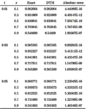
Eqs. (43) and (44) constitute the exact solutions of the Eqs. (30) and (31) respectively as given in [19]. The approximate solutions and the corresponding errors are shown in Table 1 and Table 2. Here it is to be noted that if the exact solution is not known, still we can …nd the approximate solution.
Table 1. Numarical results ofu (x; y; t)for Problem 1 whenl = n = q = 8andy = 0:1.
Table 2. Numarical results ofv (x; y; t)for Problem 1 whenl = n = q = 8andy = 0:1.
Problem 2.Here we consider the FKdV equation [13] (45) ut+ uux uuxxx+ uxxxxx= 0; with initial condition
(46) u(x; 0) = ex:
Two-dimensional di¤erential transform of Eq. (45) gives
(47) (h + 1)U (k; h + 1) =Pkr=0Phs=0U (r; h s)(k r + 1)(k r + 2) (k r + 3)U (k r + 3; s) (k + 1)(k + 2) (k + 3)(k + 4)(k + 5)U (k + 5; h) Pk r=0 Ph s=0U (r; h s)(k r + 1)U (k r + 1; s): Using Eq. (7) and the initial condition given in Eq. (46), we get
(48) U (k; 0) = 1
Substituting Eq. (48) into Eq. (47), we obtain
(49) U (k; h) = ( 1) h
k!h! ; k = 0; 1; 2; : : : ; m and h = 0; 1; 2; : : : ; n: Substituting values of U (k; h) into Eq. (7), we get
(50) u(x; t) = m X k=0 n X h=0 ( 1)h k!h! x kth= m X k=0 1 k!x k n X h=0 ( 1)h h! t h:
Letting m ! 1; n ! 1 we obtain the closed form solution.
(51) u(x; t) = ex t:
The [5=5] Padé approximant of Eq. (50) at t = 0:1 is given by
(52) R[5 5](x; 0:1) = 0:904837 + 0:452419x + 0:100537x2 1 0:5x + 0:111111x2 +0:0125672x3+ 0:000897656x4+ 0:0000299219x5 0:0138889x3+ 0:000992063x4 0:0000330688x5:
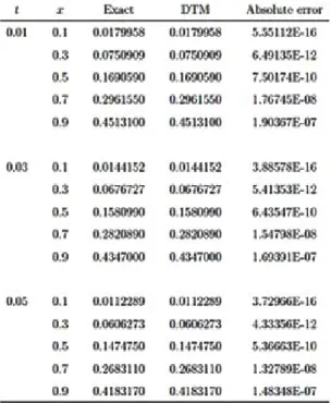
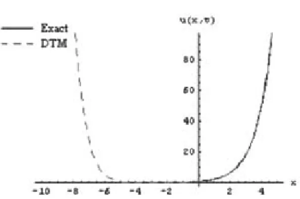
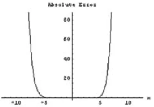
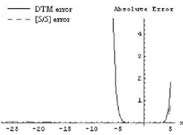
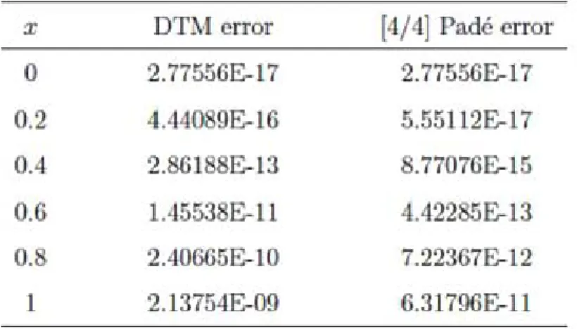
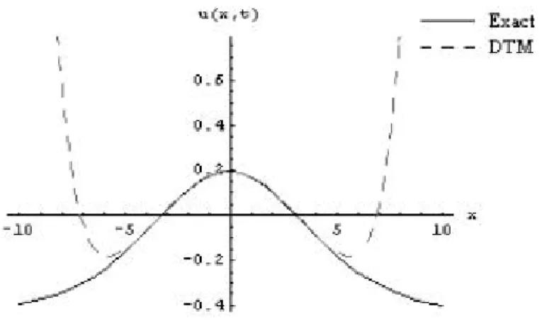
Eq. (50) is the approximate DTM solution while Eq. (51) is the exact solution of Eq. (45) which is the same as obtained by ADM [13] and can be veri…ed by substitution. Table 3 and Table 4 describe the absolute errors between the exact and approximate DTM solutions and those of Padé approximant. From the tables mentioned above it can be seen that DTM coupled with Padé Approximant has far better results than DTM alone. It can also be noted from Figure 1 and Figure 2 that although the approximate DTM solution (50) is reasonably accurate in the interval [ 4; 4], it is very poor outside the interval. It is evident from Figure 3 and Figure 4 that DTM solution (50) coupled with Padé approximant (52) is successfully used to increase the interval of convergence from [ 4; 4] to [ 10; 4].
Table 3. The absolute errors between the exact and approximate DTM solutions and those of Padé approximant for the FKdV equation (Problem 2)at m = n = 10 and t = 0:01.
Figure 1. The exact and approximate DTM solutions for FKdV equation (Problem 2)at m = n = 10 and t = 0:1.
Figure 2. The absolute error between the exact and approximate DTM solutions for FKdV equation (Problem 2) atm = n = 10andt = 0:1.
Figure 3. The exact solution and approximate DTM with [5=5] Padé approximant for the FKdV equation (Problem 2) atm = n = 10andt = 0:1.
Table 4. The absolute errors between the exact and approximate DTM solutions and those of Padé approximant for the FKdV equation (Problem 2) atm = n = 10
andt = 0:1.
Figure 4. The absolute error between the exact and approximate DTM solutions and approximate DTM with [5=5] Padé approximant for the FKdV equation (Problem 2) atm = n = 10 and t = 0:1.
Problem 3. We consider another member of class of FKdV equations, known as the Kawahara equation [18]
(53) ut+ uux+ uxxx uxxxxx= 0; with initial condition
(54) u(x; 0) = 72 169 + 105 169 sech 4 1 2p13x :
Two-dimensional di¤erential transform of Eq. (53) gives (55) (h + 1)U (k; h + 1) = (k + 1)(k + 2)(k + 3)(k + 4)(k + 5)U (k + 5; h) Pk r=0 Ph s=0U (r; h s)(k r + 1)U (k r + 1; s) (k + 1)(k + 2)(k + 3)U (k + 3; h):
Using Eq. (7) and the initial condition given in Eq. (54), the results corre-sponding to m = n = 8 are given below U (k; 0) = 0; k = 1; 3; 5; 7
(56) U (0; 0) = 33 169; U (6; 0) = 329 35644128 U (2; 0) = 105 4394; U (8; 0) = 251 1853494656 U (4; 0) = 245 456976:
Substituting Eq. (56) into Eq. (55), we obtain (57) U (k; h) = 0; kis even and h is odd
or vice versa
U (0; 2) = 6274851768040 ; U (1; 1) = 3712933780 U (0; 4) =2329808512248125719120 ; U (1; 3) =1378584918492857680 U (0; 6) = 86504159193813379337460014464 ; U (1; 5) = 511858930140907571243335744 U (0; 8) =32118388779548551051573691844006736384 U (1; 7) =19004963774880799438801409779274752 and so on. Substituting all values of U (k; h) into Eq. (7), we obtain u(x; t) = 33 169 68040t2 62748517+ 25719120t4 23298085122481 7460014464t6 8650415919381337933 + 1844006736384t 8 3211838877954855105157369+ x 3780t 371293+ 2857680t3 137858491849 1243335744t5 51185893014090757+ 409779274752t7 19004963774880799438801 + : : : + x8 251 1853494656 104517t2 28674566304592+ 236501451t4 10646665746930877456 174180752217t6 2470645290734503927044130+ 69340952777076t8 458666650966343083291998080045; or, (58) u(x; t) = 16972+105169h1 371293648t2 +137858491849244944t4 255929465070453785355238784t6 +665173732120827980358035614668912128t8 +x 36t 2197+ 27216t3 815730721 59206464t5 1514375532961265 136593091584t7 3935939243318508759515 + : : : + x 8 251 1151579520 4977t2 848359949840+ : : : + 23113650925692t8 94990134815514839735029188175 i :
Letting m ! 1; n ! 1; we obtain the closed form solution (59) u(x; t) = 72 169 + 105 169 sech 4 1 2p13 x + 36 169t : The [4=4] Padé approximant of Eq. (58) at t = 0:5 is given by
(60) R[4 4](x; 0:5) = 0:194995 0:00402483x 0:0188909x2 1 + 0:00545091x + 0:0256243x2 0:0000166058x3 0:0000392388x4 0:0000801669x3+ 0:00018847x4 :
Eq. (58) is the approximate DTM solution while Eq. (59) is the exact solution of Eq. (53), which is the same as obtained by ADM [18] and can be veri…ed by substitution. From Figure 5 and Figure 6 it can be noted that although approximate DTM solution (58) is fairly accurate in the interval [ 5; 5], it is very poor outside the interval. It is evident from Figure 7 and Figure 8 that Padé approximant (60) has been introduced e¤ectively to the approximate DTM solution (58) to enlarge the interval of convergence. In Table 5 and Table 6 we record the absolute errors between the exact and approximate DTM solutions and those of Padé approximant. From Table 5 and Table 6 it is clear that for large values of x the results of approximate DTM depreciate as compared to the small values of x. In Table 7 the approximate DTM is compared with Sinc-Galerkin Method (SGM) [18]. From the numerical results it is obvious that for the solution of the Kawahara equation, DTM is more e¢ cient than SGM.
Table 5. The absolute errors between the exact and approximate DTM solutions and those of Padé approximant for the Kawahara equation (Problem 3) atm = n = 8
Figure 5. The exact and approximate DTM solutions for the Kawahara equation (Problem 3) atm = n = 8 att = 0:5.
Figure 6. The absolute error between the exact and approximate DTM solutions for the Kawahara equation (Problem 3) atm = n = 8
Figure 7. The exact solution and approximate DTM with [4=4]
Padé approximant for the Kawahara equation (Problem 3) at
m = n = 8and t = 0:5.
Table 6. The absolute errors between the exact and approximate DTM solutions and those of Padé approximant for the Kawahara equation (Problem 3) atm = n = 8 andt = 0:1.
Table 7. The absolute errors between the exact and approximate DTM solutions and those of Padé approximant for the Kawahara equation (Problem 3) atm = n = 8 in comprasion with SGM [18].
Figure 8. The absolute error between the exact and approximate DTM with
[4=4] Padé approximant for the Kawahara equation (Problem 3) atm = n = 8
andt = 0:5.
6. Closure
In this paper, we have used DTM to …nd the exact and approximate solutions to coupled Burger’s equation. We have applied DTM with Padé approximant to a class of nonlinear …fth-order Korteweg-de Vries (FKdV) equations. This approach is simple to apply, as it does not require linearization, discretization or perturbation like other approximate methods. Further this technique requires less computational work. This con…rms our belief that the present method is very e¢ cient in applications.
The corresponding author is grateful to Higher Education Commission (HEC) Pakistan for the …nancial support. We are also thankful to the reviewers for their constructive comments.
References
1. Abolwitz M.J. and Clarkson P.A. Solitons, nonlinear evolution equations and inverse scattering. Cambridge University Press, Cambridge, 1991.
2. Esteevez P.G. Darboux transformation and solutions for an equation in 2+1 dimen-sion. J. Math. Phys. 1999;40:1406-1419.
3. Fan E.G. Darboux transformation and soliton like solutions for the Gerdjikov-Ivanov equation. J. Phys. A 2000;33:6925-6933.
4. Hirota R. and Satsuma J. CSoliton solution of a coupled KdV equation. Phys. Lett. A 1981;85:407-408.
5. Tam H.W., Ma W.X., Hu X.B. and Wang D.L. The Hirota-Satsuma coupled KdV eqaution and coupled Ito system revisited. J. Phys. Soc. Japan 2000;69:45-51. 6. Olver P.J. Applications of Lie groups to di¤erential equations. Springer, New York, 1993.
7. Bluman G.W. and Kumei S. Symmetries and di¤erential equations. Springer, Berlin, 1989.
8. Alber M.S. and Fedorov Y.N. Alberaic geometrical solutions for certain evolution equations and Hamiltonian ‡ows on nonlinear subvarieties of generalized Jacobians. Inverse Probl. 2001;17:1017-1042.
9. Cao C.W., Geng X.G. and Wang H.Y. Algebro-geometric solution of the 2+1 dimensional Burger’s equation with a discrete variable. J. Math. Phys. 2002;43:621-643.
10. Mal‡iet W. Solitary wave solutions of nonlinear wave equations. American J. Phys. 1992;60:650-654.
11. Wazwaz A.M. Abundant solitons solutions for several forms of the …fth-order KdV equation by using the tanh method. Applied Mathematics and Computation 2006;182:283-300.
12. Wazwaz A.M. Solitons and periodic solutions for the …fth-order KdV equation. Applied Mathematics Letters 2006;19:1162-1167.
13. Kaya D. An explicit and numerical solution of some …fth-order KdV equation by decomposition method. Appl. Math. Comput. 2003;144:353-363.
14. Cesar A. and Gomez S. Special forms of the …fth-order KdV equation with new periodic and soliton solutions. Applied Mathematics and Computation 2007;189:1066-1077.
15. Lei Y., Fajiang, Z. and Yinghai, W. The homogeneous balance method, Lax pair, Hirota transformation and a general …fth-order KdV equation. Chaos, Solitons and Fractals 2002;13:337-340.
16. Dehghan M., Hamidi A. and Shakourifar M. The solution of coupled Burger’s equations using Adomian-Pade technique. Applied Mathematics and Computation 2007;189:1034-1047.
17. Abdou M.A. and Soliman A.A. Variational iteration method for solving Burger’s and coupled Burger’s equations. Journal of Computational and Applied Mathematics 2005;181:245-251.
18. Kaya D. and Al-Khaled K. A numerical comparison of a Kawahara equation. Phys. Lett. A 2007;363:433-439.
19. Kansa E.J. Exact explicit time integration of hyperbolic partial di¤erential equa-tions with mesh free radial basis funcequa-tions. Engineering Analysis with Boundary Ele-ments 2007;31:577-585.
20. Nee J. and Duan J. Limit set of trajectories of the coupled viscous Burgers equations. Applied Mathematics Letters 1998;11:57-61.
21. Akylas T.R. and Yang T.S. On short-scale oscillatory tails of long-wave distur-bances. Studies in Appl. Math. 1995;94:1-20.
22. Hunter J.K. and Scheurle J. Existence of perturbed solitary wave solutions to a model equation for water waves. Physica D 1988;32:253-268.
23. Pukhov G.E. Di¤erential Transformations and Mathematical Modelling of Physical Processes. Kiev, 1986.
24. Zhou J.K. Di¤erential transformation and its Applications for Electrical Circuits. Huazhong University Press, Wuhahn, China, 1986.
25. Chen C.K. and Ho S.H. Solving partial di¤erential equations by two-dimensional di¤erential transform method. Appl. Math. Comput. 1999;106:171-179.
26. Ayaz F. Solutions of the system of di¤erential equations by di¤erential transform method. Appl. Math. Comput. 2004;147:547-567.
27. Islam S.U., Haq S. and Ali J. Numerical solution of special 12th-order boundary value problems using di¤erential transform method. Commun. Nonlinear Sci. Numer. Simulat. 2009;14:1132-1138.
28. Kangalgil F. and Ayaz F. Solitary wave solutions for the KdV and mKdV equations by di¤erential transform method.
29. Abassy T.A., El-Tawil M.A. and El-Zoheiry H. Solving nonlinear partial di¤er-ential equations using the modi…ed variational iteration Pade technique. J. Comput. Appl. Math 2007;207:73-91.
30. Momani S. and Erturk V.S. Solutions of non-linear oscillators by the modi…ed di¤erential transform method. Comput. Math. Appl. 2008;55:833-842.
31. El-Shahed M. Application of di¤erential transform method to non-linear oscillatory systems. Commun. Nonlinear Sci. Numer. Simulat. 2008;13:1714-1720.
32. Burden R.L. and Faires J.D. Numerical Analysis. PWS Publishing Company, Boston, 1993.
33. Mathews J.H. and Fink K.D Numerical Methods Using MATLAB. Prentice Hall, Delhi, 2004.
![Figure 7. The exact solution and approximate DTM with [4=4]](https://thumb-eu.123doks.com/thumbv2/9libnet/4755277.90795/19.918.236.513.216.413/figure-exact-solution-approximate-dtm.webp)
![Figure 8. The absolute error between the exact and approximate DTM with [4=4] Padé approximant for the Kawahara equation (Problem 3) at m = n = 8 and t = 0:5 .](https://thumb-eu.123doks.com/thumbv2/9libnet/4755277.90795/20.918.232.556.491.715/figure-absolute-approximate-padé-approximant-kawahara-equation-problem.webp)
