CONTINUOUS TIME COUNTERPART OF VECTOR AUTO REGRESSION OF TERM STRUCTURE DYNAMICS WITH JUMP DIFFUSION
PROCESSES A Master’s Thesis by GÜLŞAH AKSU Department of Economics Bilkent University Ankara May 2010
CONTINUOUS TIME COUNTERPART OF VECTOR AUTO REGRESSION OF TERM STRUCTURE DYNAMICS WITH JUMP DIFFUSION PROCESSES
The Institute of Economics and Social Sciences of
Bilkent University
by
GÜLġAH AKSU
In Partial Fulfilment of the Requirements for the Degree of MASTER OF ARTS in THE DEPARTMENT OF ECONOMICS BĠLKENT UNIVERSITY ANKARA May 2010
I certify that I have read this thesis and have found that it is fully adequate, in scope and in quality, as a thesis for the degree of Master of Arts in Economics.
---
Asst. Prof. Dr. Mehmet Taner Yiğit Supervisor
I certify that I have read this thesis and have found that it is fully adequate, in scope and in quality, as a thesis for the degree of Master of Arts in Economics.
---
Assoc. Prof. Dr. Refet Soykan Gürkaynak Examining Committee Member
I certify that I have read this thesis and have found that it is fully adequate, in scope and in quality, as a thesis for the degree of Master of Arts in Economics.
---
Asst. Prof. Dr. Ayse Basak Tanyeri Examining Committee Member
Approval of the Institute of Economics and Social Sciences
--- Prof. Dr. Erdal Erel
iii
ABSTRACT
CONTINUOUS TIME COUNTERPART OF VECTOR AUTO REGRESSION OF TERM STRUCTURE DYNAMICS WITH JUMP DIFFUSION PROCESSES
AKSU, GülĢah
M.A., Department of Economics Supervisor: Asst. Prof. Dr. Mehmet Taner Yiğit
May 2010
The understanding of bond yields is important for several reasons such as forecasting, monetary and debt policies, derivative pricing and investment decisions. The existence of a huge literature on this subject is a clue on how lots of researchers are trying to improve modeling of bond yields. In this paper two of such improvements are presented and discussed. The first improvement to be discussed is by Ang and Piazzesi (2003) who have found out that inclusion of macro variables to the affine term structure models provides a better fit empirically. The second improvement by Das (1998) also provides a better fitting term structure model by modeling the underlying state variable following a jump process.
iv
ÖZET
VADE YAPISI DĠNAMĠKLERĠNĠN VEKTÖR OTOREGRESYONUNUN ZIPLAMA PROSESLERĠYLE SÜREKLĠ ZAMAN KARġILIĞI
AKSU, GülĢah
Yüksek Lisans, Iktisat Bölümü
Tez Yöneticisi: Yrd. Doç. Dr. Mehmet Taner Yiğit May 2010
Bono getirilerinin anlaĢılması, öngörü yapmak, para ve borç politikaları, türev fiyatlandırması ve yatırım kararları gibi pek çok açıdan önemlidir. Bu konu ile ilgili olan literatürün fazlalığı, pek çok araĢtırmacının bono getirilerini modellemeyi geliĢtirmeye dair çabalarına bir ipucu olarak görülebilir. Bu makalede, bu yöndeki geliĢmelerden iki tanesi sunulup tartıĢılmaktadır. GeliĢmelerden ilki Ang ve Piazzesi (2003) tarafından, makro değiĢkenlerin vade yapısı modellerine katılmasının empirik dataya daha çok uyum sagladığıdır. Ġkinci geliĢme ise Das (1998) tarafından durum değiĢkenleri zıplamalar gösterirken vade yapısı modellerinin daha iyi uyum sağlaması olarak bulunmuĢtur.
v
ACKNOWLEDGEMENTS
Foremost, I would like to express my sincere gratitude to my supervisor Asst. Prof. Dr. Taner Yiğit and Assoc. Prof. Dr. Refet Gürkaynak in Bilkent University for their support of my master study and research, for their patience, motivation, and immense knowledge.
I would also like to thank Recep Yılmaz for his encouragement all through my studies. AyĢegül Dinççağ, Sezin Saraçoğulları, Fatih Cemil Özbuğday, Bilge KarataĢ and Can Kızılay also deserve special thanks as I always felt their presence throughout my study.
Last but not the least; I would like to thank my family: my father Ertugrul Aksu, my mother Filiz Aksu and my sister Deniz Aksu Arıca for supporting me throughout my life. Finally, I would like to say that I am grateful to The Scientific and Technological Research Council of Turkey (TÜBĠTAK) for supporting me for my master studies.
vi
TABLE OF CONTENTS
ABSTRACT ... iii ÖZET... iv ACKNOWLEDGEMENTS ... v TABLE OF CONTENTS ... viLIST OF TABLES ... vii
LIST OF FIGURES ... viii
CHAPTER I: INTRODUCTION ... 1
CHAPTER II: THE MODEL ... 8
2.1. Macro variables ... 9
2.2. Short rate dynamics ... 10
2.3. Term structure model with macro factors ... 10
2.4. Continuous time approximation... 11
2.5. Affine jump diffusion of the state vector ... 18
CHAPTER III: RESULTS ... 22
3.1. Estimation of term structure dynamics ... 28
3.1.1. Maximum Likelihood Estimation ... 29
3.1.2. Generalized Method of Moments Estimation ... 31
CHAPTER IV: CONCLUSION AND DISCUSSION ... 32
vii
LIST OF TABLES
1. Summary Statistics of data ... 22
2. The dependence of the short rate on macro variables ... 25
3. Descriptive Statistics ... 29
4. Continuous Time Jump Diffusion Model Estimation ... 30
5. Estimation of Discrete Time Approximation ... 31
viii
LIST OF FIGURES
1. Yield weights for the macro and macro lag model ... 26 2. Impulse response functions ... 27
1
CHAPTER I
INTRODUCTION
The understanding of bond yields is important for several reasons; according to Piazzesi (2003), there are at least four reasons for the importance of the understanding of bond yields. The first one is forecasting: yields on long-maturity bonds are risk adjusted expected values of average future short yields. The second one is monetary policy: the central banks are able to move the short end of the yield curve. The third one is debt policy: the maturity of the new bonds to issue debt is an important decision by the governments. Last one is derivative pricing and hedging. Term structure models are used to analyze the behavior of bond yields by determining the price of zero-coupon bonds. Following this reasoning, Ang and Piazzesi (2003) have investigated the term structure dynamics with macroeconomic and latent variables as state variables. Their results show that market prices of risk coefficients corresponding to the macro variables are highly significant and that macro variables explain movement at the short end and middle end of the yield curve while latent variables explain most of the variation in the long end.
Monfort et al. (2008) propose a general econometrics approach to no-arbitrage asset pricing modeling based on the historical discrete-time dynamics of
2
the factor representing the information, the stochastic discount factor and the discrete time risk neutral factor dynamics. They distinguish three modeling strategies: the direct modeling, the risk-neutral constrained direct modeling and the back modeling to model security markets and term structure of interest rates. The paper combines financial econometrics and no-arbitrage asset pricing, i.e. discrete time processes and continuous time diffusion processes. Following this modelling procedure, the main idea in the article by Ang and Piazzesi (2003) is to investigate how macro variables affect bond prices and the dynamics of the yield curve. For this purpose, the authors used a term structure model with inflation and economic growth factors with also latent variables.
According to Cox, Ingersoll, Ross (1985), risk aversion, investment alternatives and preferences of timing of consumption all play a role in determining bond prices. They used an intertemporal general equilibrium asset pricing model to study the term structure of interest rates and included factors influencing term structure of interest rates which are consistent with maximizing behavior and rational expectations. Their term structure model of interest rates measures the relationship among the yields that differ only in their term to maturity. In this respect, a complete schedule of interest rates across time embodies the market’s anticipations of future events and term structure provides a way to extract this information and to predict how changes in the underlying factors affect the yield curve. Duffie and Kan (1996) presents an arbitrage-free multifactor model of the term structure of interest rates in which the factors of the model are the yields of zero-coupon bonds of n various fixed maturities and they are observable from the current yield curve. The model by Duffie and Kan (1996) can be thought of as a multivariate version of the factor model of Cox, Ingersoll, Ross (1985).
3
Diebold et al. (2005) states that the short rate is a building block for yields of other maturities which are risk adjusted expectations of the future short rates and a joint macro-finance modeling strategy would be useful to understand the term structure of the interest rates. According to the authors, since a small number of systematic risk sources underlie the prices of the tradable financial assets, bond price information can be summarized with a few constructed variables or factors. Hence, a small set of factors and associated factor loadings that relate yields of different maturities to those factors form a structure for yield-curve models. In their paper it is stated that the bond yield factors and factor loading can be constructed by two methods. In the first method, which is also employed in Ang and Piazzesi (2003), the factors can be chosen to be the first three principal components matching empirical proxies for level ( long rate), slope (long minus short rate) and curvature (mid-maturity rate minus short- and long-rate average) and the factors are restricted to be mutually orthogonal. The factor loadings are relatively unrestricted. In the analysis by Litterman and Scheinkman (1991), most of the variation in returns on all fixed-income securities can be explained in terms of these three factors and the authors defined the loading of the bond on a factor, systematic risk in the market, by the sensitivity of the bond’s returns to the common factor. In the second method, a fitted Nelson-Siegel curve is used to present a dynamic three factor model of level, slope and curvature. The third method is the no-arbitrage dynamic latent-factor model; Ang and Piazzesi (2003) also refer to this method. In this method, linear or affine forms for the latent factors are used and the factor loadings are restricted by ruling out arbitrage strategies involving various bonds.
According to Diebold et al., by the assumption of no-arbitrage, the dynamic evolution of yields over time is consistent with the cross-sectional shape of the yield
4
curve at any point in time after accounting for risk. Therefore it is useful to include no arbitrage modeling restrictions and Ang and Piazzesi (2003) present empirical evidence such that no-arbitrage restrictions improve forecasting performance. As Ang and Piazzesi state, in the absence of a general equilibrium model for asset pricing, factor models have the advantage by only imposing no-arbitrage conditions that characterize the equilibrium in the economy. Some studies attempted to directly model the relationships between bond yields and macro variables by using vector autoregressive models with yields of various maturities together with macro variables (Estrella and Mishkin, 1997, Evans and Marshall, 1998). In these studies, the relationships between yield movements and shocks in macro variables are analyzed by using impulse responses and variance decomposition. These techniques are also applied by Ang and Piazzesi (2003).
Regarding the term structure dynamics, Piazzesi (2003) states that some discontinuous moves or jumps can be seen in the state vector, in which real interest rate and expected inflation are affine, due to macroeconomic news releases, news on financial crisis, policy moves and central bank meetings. The arrival times of these jumps can be stochastic or deterministic and the jump timing and jump size distribution can be state dependent. Related to this, Duffie and Kan (1996) state that sudden changes in perceptions of future interest rates might be modeled by allowing for surprise jumps in the state vector such as the state vector following standard jump diffusion process.
Das (1998) states that stylized facts in the bond markets suggest some jump behavior and attempts to improve bond price modeling by using jump diffusion processes. He estimates a class of Poisson-Gaussian processes allowing for jumps in interest rates. In his model, the only factor affecting bond prices is assumed to be the
5
interest rate and with the results he concludes that such jump processes provide a better fit than the diffusion models and the existing diffusion models can be enhanced by jump processes. Parallel to Duffie and Kan (1996), Das (1998) also provides an explicit derivation of the bond prices where the underlying factor follows a jump diffusion process.
In this respect, this paper aims to investigate inclusion of such jumps into the model by Ang and Piazzesi (2003) where the process of latent factors will be assumed to follow Gaussian AR(1) which is the discrete time counterpart of Ornstein-Uhlenbeck process. The process of macroeconomic variables can be modified by adding the stochastic jump process to the Ornstein-Uhlenbeck process assumed in Ang and Piazzesi (2003). In the next sections, the results of both Ang and Piazzesi (2003) and Das (1998) will be discussed as further improvements to theexisting bond pricing models.
Merton (1976) states the validity of Black Scholes solution for derivative prices depends on whether or not stock price changes by a small amount in a short time interval which can be modeled by standard geometric brownian motion. However, this might not be the case and such a situation can be modeled by using stochastic jump processes defined in continuous time which allows for a positive probability of extraordinary changes in stock prices no matter how small the time interval is. This kind of abnormal vibrations in stock prices can be due to arrival of important new information about the stock. According to Merton (1976), a prototype for the jump component is a Poisson driven process where the poisson distributed event is the arrival of important information about the stock. The arrival times are independent and identically distributed.
6
Piazzesi (2001) incorporates macro variables in a term structure model where policy related events and releases of macroeconomic news are modeled as jumps. According to Piazzesi, at high data sampling frequencies, information about the exact timing of policy-related events can be used to improve bond pricing and to identify monetary policy shocks. The author estimated the model by the method of simulated maximum likelihood extended to the case of jumps. Using the fact that the FED conducts monetary policy by targeting the overnight rate in the federal fund market, the target is modeled as a pure jump process. The model in Piazzesi uses the state variable vector including the target rate, some macro variables, analyst forecasts of those macro variables and unobservable (latent) variables, including the short rate and the spread between the short rate and the target rate. The general dynamics of the state vector in this model follows a jump diffusion process
( )
( )
() ( ) )(t X t dt X t dW t dJ t
dX
where J is a pure jump process, W is a vector of Brownian motions, μ is the drift and ζ is the volatility. The drift and the variance-covariance term are linear functions of the state, which allows for conditional heteroscedasticity and the jumps can capture macroeconomic jump effects such as policy events caused by a financial crisis and macroeconomic releases. In the model of Piazzesi jumps occur only when macroeconomic variables are announced. Johannes (2004) has found that jumps only occur when the announcements contain significant unexpected components. Johannes states that if the short rate is observed continuously then
r Z r where s t s t r r
lim and Z is the jump size, η is the jump time. However, in practice, observations are available only discretely and this limit cannot be computed. Therefore he uses a discrete time example:
7 t t t t t t t r r r J Z r ( ) ( )
where Jt=1 with probability λΔ, t ~ N(0,)and ~ (0, )
2 Z t N
Z
.In the following section, the model by Ang and Piazzesi (2003) will be investigated. Representing their model in continuous time, jump diffusion model for the state vector will be introduced. In the third section results of Ang and Piazzesi paper and possible improvements of jump diffusion process representation will be discussed. The conclusions will be presented in the last section.
8
CHAPTER II
THE MODEL
Ang and Piazzesi (2003) investigate the affects of macro variables on bond prices and the dynamics of the yield curve in a discrete time model. For this purpose, they use factor representation of the pricing kernel, which by definition prices all bonds in the economy, where the factors are observed macro variables and unobserved variables. According to the authors, since macro factors are correlated with yields, including these factors may lead to better forecasting models. They investigated whether the unobservable factors of the multi-factor term structure models can be explained by macro variables and also how the effects of latent factors change when macro variables are incorporated into such models.
Their methodology allows characterizing the behavior of the entire yield curve in response to macro shocks rather than just the yields included in the VAR. It also allows making a direct comparison of macro variables with latent yield factors. The method of variance decomposition can be used to estimate the proportion of term structure movements attributable to observable macro shocks and other latent variables. Their approach also retains the tractability of the VAR approaches, since they estimate VAR subject to nonlinear no-arbitrage restrictions.
9
The authors used a Gaussian term structure model; therefore it is a VAR model. Their model is a special case of discrete-time versions of the affine class introduced in Duffie and Kan (1996). Bond prices are exponential affine functions of the underlying state variables, where some of the state variables are observed macroeconomic aggregates. The Gaussian term structure model allows them to compute impulse responses and variance decompositions easily.
They obtain the measures of inflation and real activity by extracting principal components of two groups of variables that are selected to represent measures of price changes and economic growth. Then they estimate the model with three latent factors in addition to the macro variables as state variables.
2.1. Macro variables
The authors sorted the macro variables in two groups: inflation measures and real activity measures. The inflation measures are based on the CPI, the PPI of finished goods and spot market commodity prices. The real activity measures are based on the index of Help Wanted Advertising in Newspapers, unemployment, the growth rate of employment and the growth rate of industrial production. The first principal component of each group of variables is extracted to reduce the dimensionality of the system. They estimate a bivariate process with 12 lags for the macro factors: 0 0 12 12 0 1 1 0 t t t t f f u f
where ft0
fto,1fto,2
' are the extracted macro factors and 1to12and are2
10 2.2. Short rate dynamics
As also discussed by Duffie and Kan (1996) affine term structure models are based on a short rate equation and an assumption on risk premia. The affine term structure models specify the short rate to be an affine function of underlying factors, in which the factors themselves follow affine processes. The authors modeled the short rate in the following manner:
u t t
t X X
r
0
11' 0
12'where the latent factors Xtu is specified to be orthogonal to the macro factors Xt0, so that the short rate dynamics of the term structure model can be interpreted as a version of the Taylor (1993) rule, which states that movements in the short rate are traced to movements in contemporaneous macro variables and an orthogonal shock
(v ) which is not explained by the macro variables, with the errors t vt Xtu ' 12
being
the unobserved factors. In order to identify the latent factors the authors used the restrictions from no-arbitrage and they estimated the short rate dynamics with ordinary least squares since 0
t
X and u t
X are independent.
2.3. Term structure model with macro factors
The authors combine observable macroeconomic variables with unobservable or latent factors. They assume that the observable vector contains current and past levels of macroeconomic variables, Xto
fto',fto1',,fto13'
, and the unobservable vector only contains contemporaneous latent yield factors,u t u t f
X ,. Then the dynamics of the state variableXt
Xto' Xtu'
is written as a Gaussian VAR (1) process:t t
t X
11
with
t
uto',0,,0,utu
', where utoand utuare the shocks to the observable and unobservable factors. The latent factors,Xtu, in their models are AR(1) withu t u t u t X u X
1where utu ~ IIDN
0,I is a 3 dimensional shock vector.2.4. Continuous time approximation
The diffusion approximation of AR(1) model can be obtained as follows (Gourieroux, Jasiak, 2001): u t u t u t X u X 1
u t u t u t u u X 2 1 u t u t u t u t u t u u u u X 1 1 2 2 1 Xtu utu 1 1 Assuming exp( k ): u t u t u t X u X 1 1
k
Xtu k 2 utu 1 1 u t u t u t u t X k X u X * By letting 𝛿 = 𝑑𝑡, 𝑋𝑡+𝛿𝑢 − 𝑋𝑡𝑢 = 𝑑𝑋𝑡𝑢 and 𝑊𝑡 as the Wiener process with increment 𝑊𝑡+𝛿 − 𝑊𝑡 = 𝑑𝑊𝑡 we reach to the Ornstein-Uhlenbeck process:
t u t u t kX dt dW dX *
Similarly for a Gaussian VAR(1) model as above, the diffusion approximation can be obtained by subtracting Xt1 from both sides:
12 t t t X X 1 t t t t t X X X X 1 1 1
* t t t I X dt dW dX where 𝑊𝑡∗ is a vector Brownian motion.Monfort et.al. (2008) name the new information, ωt, in the economy at date t as factors or state variables, which can be observable, partially observable or unobservable. Their paper defined the historical dynamics of the factor variables by their joint distribution over a finite horizon or by the conditional Laplace transform, conditional on the overall information at time t:
t
t
t
t u E u
| exp ' 1 |
and the conditional log-Laplace transform:
t
u|t
log
t
u|t
Monfort et.al. (2008) consider the following assumptions for the stochastic discount factor denoted by Mt in their paper:
Any payoff 𝑔 𝜔𝑠 of the space of square integrable functions delivered at s
has a unique price at any time t<s for any overall information at time t, 𝜔𝑡, denoted by 𝑝𝑡 𝑔 𝜔𝑠
Law of one price holds and the pricing function is continuous
There is no arbitrage opportunity: at any time 𝑡 ∈ 0, 𝑇 it is impossible to
form a portfolio such that its price at time t is non-positive, its payoffs at some points in time are non-negative and there is at least one point in time where the net payoff is strictly positive with strictly positive conditional probability at time t.
As Ang and Piazzesi (2003) state, the assumption of no-arbitrage implies the existence of an equivalent martingale measure, risk neutral measure, Q such that the
13 equality Pt EtQ
ertXt1
is satisfied, where P is the price, X is the payoff of the asset and the expectation is taken under the risk neutral probability measure. This assumption also implies the existence of the Radon – Nikodym derivative and denoting the Radon - Nikodym derivative, which converts the risk-neutral measure to the data generating measure, byt1for any random variable Z;
1 1 1 t t t t t Q t Z E Z E holds. Any asset in the economy including nominal bonds
can be priced in this manner. The authors assume thatt1follows the log-normal
process with the source of uncertaintyt :
1 ' ' 1 2 1 exp t t t t t t
and parameterize the time-varying market prices of risktas an affine process:
t t 0 1X
The above two equations determine how shocks in the factors are affecting the yields by the shock in the underlying state variablesX to the Radon – Nikodym t derivative.
Ang and Piazzesi (2003) then define the pricing kernel mt1 as:
t t t t r m 1 1 exp ' 0 1' ' 1 2 1 exp t t Xt t tIn Monfort et al. (2008), the risk neutral dynamics are defined as another joint distribution of the overall information at time T of the state variables as:
1 1 , 1 1 , 1| t t t t t t t t t Q t M E M d 14
Since the price at time t of a zero coupon bond maturing at t+1 is
t1 exp
rt1
B
,1
Et Mtt
Then the above equation for risk neutral dynamics can be written as:
t1| t
exp
t1 t,t1
t1Q
t r M
d
Therefore to be able to reach the pricing equation, the following equality should hold:
t t
Q t t t t t t Q t d f f | | | 1 1 1 In terms of Ang and Piazzesi (2003), the above term equals to
t t 1 .
Monfort et al then show that assuming that the stochastic discount factor has exponential affine form it can be written as:
t
t
t t t
t
t t
M ,1 1 exp '1 where 𝛼𝑡 𝜔𝑡 denotes the factor loadings or sensitivity vector.
Following Monfort et al, by using the price at time t of a zero coupon bond maturing at t+1 and the log-Laplace transform, the following equalities hold:
t
t
t t
t t tM r E ,1 exp 1 exp
1
1
1 1 ,t t t exp t t d r M
1
1 1 1 , exp t Q t t t t r d M Since the probability distribution function of the risk neutral distribution of wt with respect to the corresponding historical distribution is a P martingale, i.e.
15
1 1 1 1 t T t Q t t dP d E dQ E Then: t t t T dz d ' t t t t T dt dz d ' ' 2 1 log and the solution is:
t u u
t u u T du dz 0 ' 0 ' 2 1 exp Therefore the continuous time version of the stochastic discount factor is:
1 1 1 ' 2 1 , exp 12 t t t t t t u u u u t t r du du dz M or
r
dt dW M d t ' ' 2 1 log and the discrete time equivalent is:
1
' ' 1 1 ,t exp t 12 t t t t t r M This equation is the same as in Ang and Piazzesi (2003) when the short rate dynamics is replaced into the equation. The equation above is also of the form:
𝑒𝑥𝑝 𝛼𝑡(𝜔𝑡)′𝜔𝑡+1+ 𝛽𝑡(𝜔𝑡)
when both the short rate dynamics and the time varying market prices of risk is written in an open form as functions of the state variables.
The nominal pricing kernel in Ang and Piazzesi (2003) prices all nominal assets in the economy, implying that the price of an n+1 period zero coupon bondptn1can be computed by:
n
t t t n t E m p p 1 1 116 For a one period bond:
t
t
t
t
t E m r X
p1 1 exp exp
0
1'Letting A1 0andB1
1, the price of an n-period bond isptn exp
An Bn'Xt
. The continuously compounded yield ytnon an n-period zero coupon bond is therefore: t n n n t n t A B X n p y log 'whereAn An n andBn Bn n. A and n Bn follow the differential equations
0
0 1 ' ' 2 1 ' n n n n n A B B B A ' ) ( ' ' 1 1 1 n n B BTherefore the yields are affine functions of the state variables and the weightsB represent the initial response of the yields from shock to the factors. n
The continuous time solution of this term structure can be represented by first defining the state variable process (𝑋𝑡) following Ornstein-Uhlenbeck diffusion process and the short interest rate 𝑟 as an affine function of the state variables.
t
t t I X dt dW dX
t x h
x r , 'The pricing kernel is assumed to follow the diffusion process
'
, 0 1
M rdt dw M
dM
which can be simplified by Ito’s lemma to the following process
r
dt dW M d t ' ' 2 1 log Since the pricing kernel follows geometric Brownian motion,
T T
T m v EM 2 1 exp 17
where mT and vT are respectively the mean and the variance of the log-pricing kernel. Denoting 𝐹 = Φ − 𝐼 the state variable and pricing kernel processes can be
combined as follows dW dt dt X M F h X M d ' ' 2 1 log 0 ' 0 log Let F h F 0 ' 0 ~ , ~ 12 ' and
~ ' . Then mT and vT are found as
T T T F T t dt X M T F h M E m 0 ~ ~ 0 0 ~ exp log exp ' log
M
h F
T t
F
T t
dt h v T T T
0 ~ ~ exp ' exp ' log varDenoting P(0,T) as the price of zero coupon bond at maturity T, expectation of pricing kernel at the maturity date is the price
P
0,T EMT exp
mT 12vT
T F T t dt X M T F h 0 ~ ~ 0 0 ~ exp log exp '
h
F T t F T t dt h T 0 ~ ~ exp ' exp ' 2 1
AT BT X
expHence the yields (𝑦𝑡𝑇) are affine in the state variables
n i i t i T t t T t T B X t T t T A y 1 ,18 2.5. Affine jump diffusion of the state vector
Duffie, Kan (1996) state that one can maintain the affine yield-factor model with a standard jump-diffusion model for the state vector X based on the infinitesimal generator 𝒟∗ defined as follows:
h x f x X X f E t x Df t h t h | lim , 0
t
x
t
t t t DF X t dt F X t X dW dp , ,
, '
2 1 , , ,t F x t F X t x tr F x t x x x DF t x t xx
x t DF
x t
F
x z t
F
x t
dv
z F D D
, , , , * (1)where 𝑝𝑡 = 𝐹 𝑋𝑡, 𝑡 is the zero coupon price process with fixed maturity date T, the arrival intensity of jumps in X at time t is denoted by the affine function 𝜆: 𝐷 → ℝ+
and the distribution of jumps is denoted by the fixed probability measure v on ℝ𝑛. They find that the solution to this partial differential equation has an exponential affine form:
x t
a
T t
bT t
x
F , exp
Duffie, Pan and Singleton (1999) define affine jump-diffusion by fixing a probability space Ω, ℱ, 𝑃 and an information filtration ℱ𝑡 , as a Markov process in some state space 𝐷 ⊂ ℝ𝑛 solving the following stochastic differential equation:
t
t t tt X dt X dW dZ
dX
where W is a standard Brownian motion in ℝ𝑛; 𝜇 is affine on D and 𝜇: 𝐷 → ℝ𝑛 , 𝜎: 𝐷 → ℝ𝑛×𝑛 and 𝜎𝜎′ is affine on D, Z is a pure jump process whose jumps have a probability distribution ν on ℝ𝑛 and the arrival intensity is 𝜆 𝑋
𝑡 : 𝑡 ≥ 0 for some
0,
: D
. As discussed in Duffie and Kan (1996) with the infinitesimal generator D of the Lévy type defined as a function f :D which is bounded C219
with bounded first and second derivatives, the Markov process X can also be represented as
, '
2 1 , , ,t f x t f x t x tr f x t x x x Df t x xx
x n
f
xz,t
f x,t
dv
z
Cont and Tankov (2004) state that a Lévy process of jump-diffusion type is composed of a Gaussian component (Wt) and a jump component of compound
Poisson type
t N i i Y 1has the form:
Nt i i t t t W Y X 1 (2)where
Nt t0 is the Poisson process counting the jumps of X, Y are i.i.d. jump isizes and
t N i i Y 1is a compound Poisson process with intensity .
Merton (1976) states the validity of Black-Scholes solution for derivative prices depends on whether or not stock price changes by a small amount in a short time interval which can be modeled by standard geometric Brownian motion. However, as the last financial crisis showed once more, this might not be the case and such a situation can be modeled by using stochastic jump processes defined in continuous time which allows for a positive probability of extraordinary changes in stock prices no matter how small the time interval is. This kind of abnormal vibrations in stock prices can be due to arrival of important new information about the stock. According to Merton (1976), a prototype for the jump component is a Poisson driven process where the poisson distributed event is the arrival of important information about the stock. The arrival times are independent and identically
20
distributed. Denoting λ as the mean number of arrivals per unit time and O(h) as the
asymptotic order symbol with ψ(h) = O(h) and lim 0 ( ) 0
h h h , the probability
of an event occurring during time interval h can be written as: Prob(event does not occur in (t,t+h)) = 1 – λh + O(h)
Prob(event occurs in (t,t+h)) = λh + O(h)
Prob(event occurs more than once in (t,t+h)) = O(h)
Merton defines the stochastic differential equation for the Poisson driven process as:
dt dZ dqS
dS
where
is the expected return on stock, dZ is the standard Gauss Wiener process with mean zero and variance t, q(t) is independent Poisson process, ζ2variance of the return conditional on number of arrivals of important new information. κ = ε (Y-1) where (Y-(Y-1) is the random variable percentage change in stock price if the poisson event occurs and ε is the expectation operator over the random variable Y. The solution to this differential equation is:
( )
( ) 2 exp ) ( 2 n Y t Z t S t S where Y(n) = 1 if n=0 and
n j j Y n Y 1 )
( if n1 and n is Poisson distributed with
parameter λt. In other words, Merton (1976) assumes Lévy process of jump-diffusion type with jump sizes in the log-price (Xt) having a Gaussian distribution:
, 2
~ N
Yi . Therefore the probability density of Xt satisfies:
0 2 2 2 2 2 2 ! 2 exp k k t t k t k k t k t x t e x p 21
In this representation excluding the drift in (2) there are four parameters to estimate: diffusion volatility (ζ), jump intensity (λ), mean jump size (μ) and standard deviation of the jump size (δ). As Cont and Tankov (2004) state, the tails of this probability density are heavier than Gaussian.
22
CHAPTER III
RESULTS
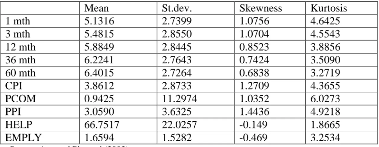
Ang and Piazzesi (2003) used data on zero coupon bond yields of maturities 1 and 3 months from FAMA CRSP Treasury Bill files and maturities of 12, 36, and 60 months from FAMA CRSP zero coupon files from June 1952 to December 2000. The summary statistics of the data shows that the excess kurtosis of the yields decreases with maturity however the authors state that for the first-differenced yields the excess kurtosis is higher such as 19.44 for the 1-month yield. Hence, the evidence for a normal distribution of yields is rejected.
Table 1. Summary statistics of data
Mean St.dev. Skewness Kurtosis
1 mth 5.1316 2.7399 1.0756 4.6425 3 mth 5.4815 2.8550 1.0704 4.5543 12 mth 5.8849 2.8445 0.8523 3.8856 36 mth 6.2241 2.7643 0.7424 3.5090 60 mth 6.4015 2.7264 0.6838 3.2719 CPI 3.8612 2.8733 1.2709 4.3655 PCOM 0.9425 11.2974 1.0352 6.0273 PPI 3.0590 3.6325 1.4436 4.9218 HELP 66.7517 22.0257 -0.149 1.8665 EMPLY 1.6594 1.5282 -0.469 3.2534
23
Johannes (2004) compares the unconditional and conditional nonnormalities in interest rates with analogs generated by diffusion models to test for presence of jumps and his findings indicate that the diffusion models fail to generate nonnormalities consistent with those of observed Treasury rates. This is due to the fact that diffusion models assume the increments are approximately normal over short time intervals while the increments of actual data are very nonnormal. He also finds that the jump-diffusion model generates conditional and unconditional kurtosis consistent with data and introducing jumps to such models is important. This improves the adequacy of the statistical model, which can be examined by estimating the model parameters from the time series of asset returns and then comparing the statistical properties of the estimated model with the properties of the observed returns (Cont and Tankov, 2004).
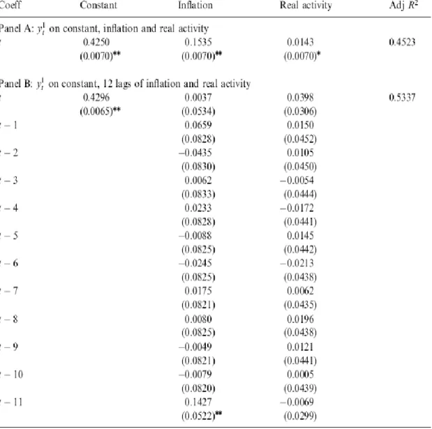
Ang and Piazzesi (2003) inferred the unobservable factors from the yields using the fact that yields are functions of the state variables and estimated the term structure model by first estimating the dynamics of the macro factors and the parameters of the short rate equation by ordinary least squares. They estimated the short rate dynamics of both the simple Taylor rule, Macro Model, and the forward looking Taylor rule, i.e. full lagged Taylor rule, Macro Lag Model. As a second step they estimate the remaining parameters of the term structure model holding all pre-estimated parameters fixed. The following table presents the regression results.
The results from Table 2 by Ang and Piazzesi (2003) show that macro variables have explanatory power for yield curve movements with an adjusted R2 of 45% and 53% for the estimated Taylor rule and the estimated forward looking Taylor rule, respectively. The results also find that the optimal Schwartz (BIC) choice is the simple Taylor rule.
24
The results by Ang and Piazzesi (2003) also show that when the model is estimated without any macro variables, i.e. only with the yields, the time variation in risk premia is mainly driven by the first and third unobservable factors or the level and curvature of the yield curve respectively.
The estimates of Macro and Macro Lag Model show that market price of risk coefficients corresponding to inflation and real activity are highly significant and hence the observable macro factors drive time variation in risk premia however their roles are dependent on the details of the model specification. The prices of risk control how the variation of longer yields respond relative to the short rate. Results show that since time varying prices of risk for inflation and real activity are negative in Macro Model, the initial shocks are larger across the yield curve.
25
Table 2. The dependence of the short rate on macro variables
Source: Ang and Piazzesi (2003).
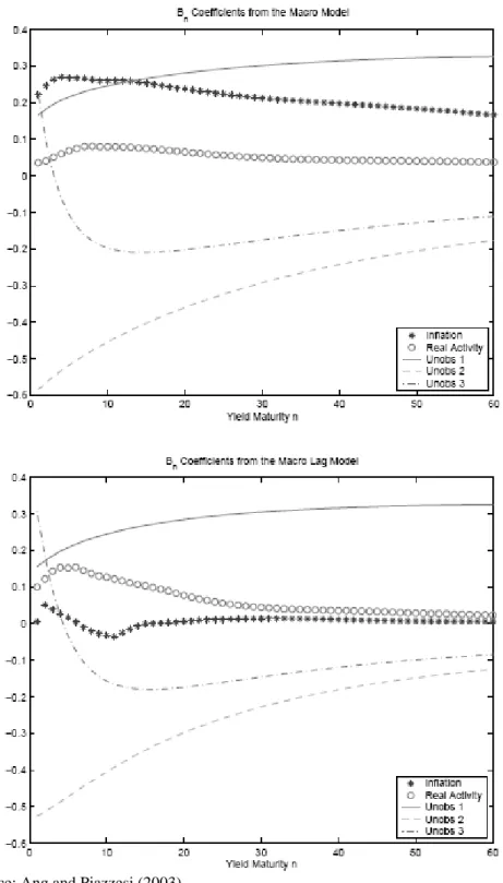
The estimation results for the weightsB in figure 1 from Ang and Piazzesi n (2003) show that the unobservable factor 1 is almost horizontal and can hence be named as level. The second and third unobservable factors are slope and curvature factors respectively and these factors are named the same for both Macro and Macro Lag Models. TheB coefficient corresponding to inflation show that inflation mostly n
affects short yields and less long yields. TheBn coefficient corresponding to real activity is much lower than for inflation and affect the yield curve weakly.
26
Figure 1. Yield weights for the macro and macro lag model
27 Figure 2. Impulse response functions
Source: Ang and Piazzesi (2003).
Figure 2, shows the impulse responses of 1 month (top row), 12 months (mid row) and 60 months (last row) yields from unrestricted VAR(12), Macro and Macro Lag models. In the figure, the initial impulse response corresponds to 1 month on the x-axis and impulse responses are given in terms of annualized percentages for a shock of one standard deviation.
The figure shows that for the unrestricted VAR(12) the response of yields to real activity shocks is slightly smaller than the response to inflation shocks and smaller than the impulse responses for Macro and Macro Lag models.
28
In the Macro model, the effect of inflation shock is much larger than the effect of real activity and both effects are hump shaped. However for Macro Lag model, there is little hump shape and the effects of inflation shocks is much smaller than the Macro model for 60 month yields. This result is due to the different estimates of the time varying price of risk for the two models. The authors also point out that lower or more negative prices of risk have higher and positive impacts from the macro factors to the long yields, i.e. higher the magnitude of the impulse responses.
In order to compare the forecasts across the two models, authors use Root Mean Squared Error of actual and forecasted yields. Their results show that when cross-equation restrictions from no arbitrage are imposed, the forecasting performance increases and the forecasts of the Macro model are much better than the Macro Lag model. Their results also show that inflation accounts mostly for the dynamics of the slope factor.
3.1. Estimation of Term Structure with jumps
In this section, two statistical estimation methods, specifically maximum likelihood estimation and generalized method of moments estimation, for the term structure of interest rates will be discussed. As Cont and Tankov (2004) state, all estimation procedures are maintained by optimizing a certain criterion and choose the model parameters within this respect. In maximum likelihood estimation method, the criterion is to maximize a likelihood function to estimate the model parameters. There are a few Levy processes for which the likelihood function is available in a closed form, which is the case if the jump size is Gaussian as in the model by Merton (Cont, Tankov, 2004). In generalized method of moments the criterion is
29
based on the moments of the distribution of the variables in the model. Different than the likelihood estimation where the likelihood function is not always available in a closed form, the expressions of moments are always available in closed form as a function of model parameters and can be obtained via the characteristic function. The estimators can be constructed based on these moments.
3.1.1. Maximum Likelihood Estimation
Das (1998) examines the role of jump diffusions in modeling the term structure of interest rates. The author estimated the following mean-reverting interest rate process with jumps, assuming that all factors determining the bond value are captured by this equation, by using daily data on the Fed funds rate for the period January 1988 to December 1997.
r
dt dz Jd (h)dr
where is the central tendency parameter for the interest rate r reverting at rate ,
2
is the variance of the diffusion,
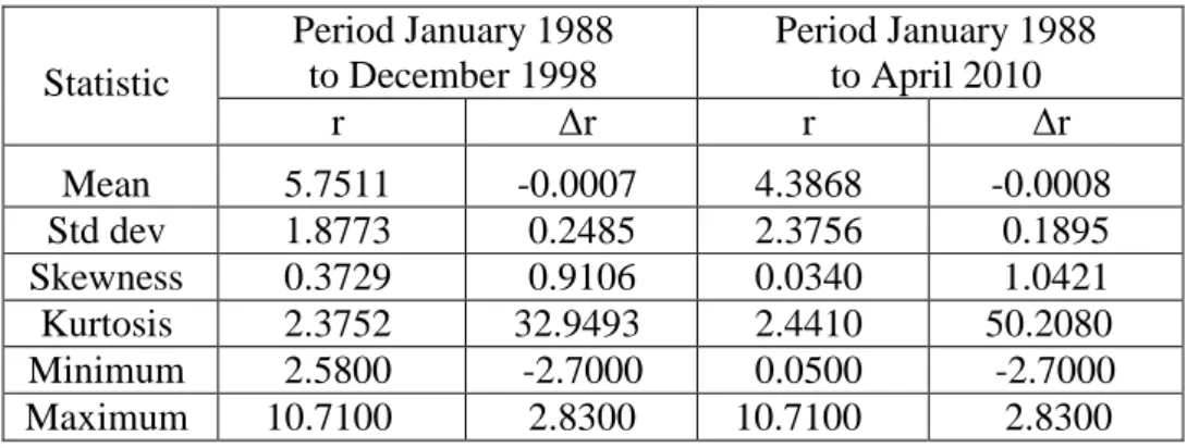
is the Poisson process with arrival frequency h, denoting the number of jumps per year and J is the jump size.In table 3, the summary statistics of the short interest rate is provided for both the period in the paper by Das (1998) and an updated period of January 1988 to April 2010. The data is obtained through the web site of Federal Reserve.
Table 3. Descriptive Statistics
Statistic Period January 1988 to December 1998 Period January 1988 to April 2010 r Δr r Δr Mean 5.7511 -0.0007 4.3868 -0.0008 Std dev 1.8773 0.2485 2.3756 0.1895 Skewness 0.3729 0.9106 0.0340 1.0421 Kurtosis 2.3752 32.9493 2.4410 50.2080 Minimum 2.5800 -2.7000 0.0500 -2.7000 Maximum 10.7100 2.8300 10.7100 2.8300
30
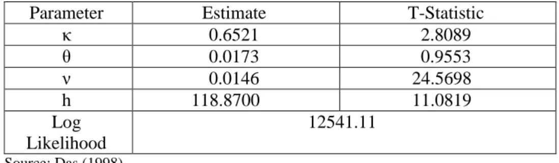
The observed leptokurtosis is a strong motivation for the use of jump models. By using the maximum likelihood method, Das estimates the continuous time process using the continuous time transition density. He also provides a derivation of bond prices under the jump-diffusion model; the bond prices are exponentially affine in the interest rate under the risk neutral probability measure.
)] ( ) ( exp[ ) , (r A rB P
The results by Das (1998) confirm that the jump parameters are statistically significant (table 4). The parameter value of h indicates a large number of jumps in the data. The positive skewness in the data is captured by the parameter ψ.
Table 4. Continuous Time Jump Diffusion Model Estimation
Parameter Estimate T-Statistic
κ 0.6521 2.8089 θ 0.0173 0.9553 ν 0.0146 24.5698 h 118.8700 11.0819 Log Likelihood 12541.11 Source: Das (1998).
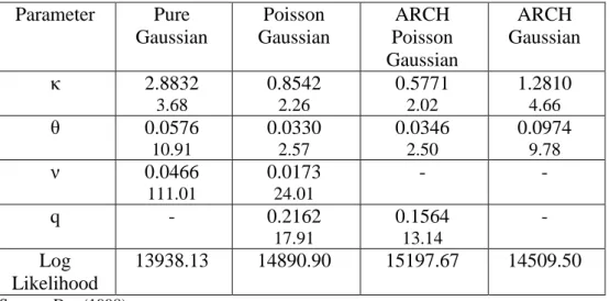
Das (1998) also estimates the model by a discrete time approach with Bernoulli approximation, in which the jumps are normally distributed. He also compares different models with this discretization, namely, a pure-Gaussian model, the Poisson-Gaussian model, an Poisson-Gaussian model and a pure ARCH-Gaussian model. The results (table 5) by Das show that the volatility of ARCH-Gaussian part decreases when jumps are introduced to the pure-Gaussian model, i.e. the parameter v takes a higher value in the Poisson Gaussian model. The parameter denoting the probability of a jump on any day, q, takes the value 0.2162 in the Poisson-Gaussian model and 0.1564 in the ARCH-Poisson-Gaussian model. This implies that some of the jumps are accounted by stochastic volatility and hence a combined ARCH-Poisson-Gaussian model captures the features of the data better.
31
The mean reversion coefficient, κ, drops when jumps are added to the pure-Gaussian model, implying that jumps provide a source of mean-reversion.
Table 5. Estimation of Discrete Time Approximation Parameter Pure Gaussian Poisson Gaussian ARCH Poisson Gaussian ARCH Gaussian κ 2.8832 3.68 0.8542 2.26 0.5771 2.02 1.2810 4.66 θ 0.0576 10.91 0.0330 2.57 0.0346 2.50 0.0974 9.78 ν 0.0466 111.01 0.0173 24.01 - - q - 0.2162 17.91 0.1564 13.14 - Log Likelihood 13938.13 14890.90 15197.67 14509.50 Source: Das (1998).
3.1.2. Generalized Method of Moments
Compared to the Maximum Likelihood estimation, this method is easier to implement and can be modeled more generally. Das (1998) estimates two models; a pure diffusion model and the jump diffusion model. The following results of Das (1998) show that the mean-reverting parameter increases when jumps are allowed, a contradicting result with the maximum likelihood estimation. The volatility of Brownian part also increases when jumps are introduced to the pure-diffusion process. Das concludes that the jump diffusion model provides a better fit than the pure diffusion model.
Table 6. Generalized Method of Moments Estimation
Pure-diffusion model Jump-diffusion model Parameter Estimate T-stat Estimate T-stat
κ 2.6880 3.69 3.0992 4.09
θ 0.0593 10.82 0.0580 12.22 ν 0.0387 11.13 0.0447 10.82
32
CHAPTER IV
CONCLUSION AND DISCUSSION
In this paper the term structure model proposed by Ang and Piazzesi (2003) and Das (1998) are summarized and discussed. Ang and Piazzesi investigate the effects of macro variables on bond prices and the dynamics of the yield curve. Although there have been some attempts to study the relationship between bond yields and macro variables using vector autoregressive models, including the paper by Ang and Piazzesi, they mostly allow for unidirectional dynamics, i.e. macro variables determine yields but not the reverse. This is also mentioned in Diebold et al. (2005) in which a bidirectional characterization of the dynamics is modeled and their results show that although the causality from the macro variables to yields is stronger than the reverse, it might still be important to consider the bidirectional relationship. The results of Ang et al. (2004) is that the bidirectional system accounts half of the variation of long yields to macro variables, which is not the case when only unidirectional dynamics are considered such that macro variables explain only a small portion of variation in long yields. Ang and Piazzesi (2003) find that the unobservable factors account for most of the variation in the long end of the yield
33
curve and macro variables explain movements at the short end and middle end of the yield curve, therefore the results of this paper can be improved by also considering the bidirectional dynamics while still imposing the no-arbitrage restriction.
Das (1998) provides an attempt to the use of jump diffusion processes in bond pricing. His model is based on the assumption that all factors determining the bond value are captured by the interest rate following a jump diffusion process. Das concludes that introducing jumps to the diffusion process of interest rates improves the model fit. He also provides an explicit derivation of bond prices under such assumptions, which is stated more generally in Duffie and Kan (1996).
In order to be able to describe the economic sources of the shocks in factors and the effects on the behavior of the yield curve, modeling the macro variables and latent factors also requires to take into account macroeconomic dynamics sufficiently. Although Ang and Piazzesi (2003) deals with this modeling successfully, their work can still be improved by considering possible jumps in the macro variables. In this respect, Piazzesi (2005) explored the role of macroeconomic variables in a no-arbitrage affine model by using the Federal Reserve’s interest-rate target as the key observable factor. According to this model the short rate is the sum of the target and short-lived deviations from the target and the target follows a pure jump process whose jump probabilities depend on the policy meetings and latent factors. The results show that considering macroeconomic information reduces the pricing errors. This model is built on jumps with deterministic jump times, however further improvement can be achieved by also using stochastic jump times additionally, which is introduced in Duffie and Kan (1996). According to Duffie and Kan, sudden changes in perceptions of future interest rates such as due to crisis periods, might be modeled by allowing for surprise jumps in the state vector by a
34
standard jump diffusion model for the state vector. Since such unexpected events occur commonly in financial markets, the model by Ang and Piazzesi might be developed further by bearing such aspects.
35
REFERENCES
Ahn, C.M., Thompson, H.E., (1988): “Jump-diffusion processes and the Term Structure of Interest Rates”, The Journal of Finance XLIII, 155-174.
Ang, A., Dong, S., Piazzesi, M., 2004. No-arbitrage Taylor rules. Working paper, University of Chicago.
Ang, A., Piazzesi, M., 2003. A no-arbitrage vector autoregression of term structure dynamics with macroeconomic and latent variables. Journal of Monetary Economics 50, 745-787.
Cont, R., Tankov, P., 2004. Financial Modelling with jump processes. US: Chapman & Hall/CRC.
Cox, J.C., Ingersoll, J.E., Ross, S.A., 1985a. An intertemporal general equilibrium model of asset prices. Econometrica 53, 363-84.
Cox, J.C., Ingersoll, J.E., Ross, S.A., 1985a. A theory of the term structure of interest rates. Econometrica 53, 385-408.
Das, S. R., 1998. Poisson-Gaussian processes and the bond markets. NBER Working paper.
Diebold, F. X., Piazzesi, M., Rudebusch, G. D., 2005. Modeling bond yields in finance and macroeconomics. American Economic Review 95, 415-420. Diebold, F.X., Rudebusch, G.D., Aruoba, S.B., 2005b. The macroeconomy and the
yield curve: A dynamic latent factor approach. Journal of Econometrics. Duffie D., Kan, R., 1996. A yield factor model of interest rates. Mathematical
Finance Vol. 6, no.4, 376-406.
Estrella, A., Mishkin, F.S., 1997. The predictive power of the term structure of interest rates in Europe and the United States: implications for the European central bank. European Economic Review 41, 1375-1401.
36
Evans, C.L., Marshall, D.A., 1998. Monetary policy and the term structure of nominal interest rates: evidence and theory. Carnegie-Rochester Conference Series on Public Policy 49, 53-111.
Gourieroux, C., Jasiak, J., 2001. Financial Econometrics. UK: Princeton University Press.
Johannes, M., (2004): “The statistical and economic role of jumps in continuous-time interest rate models”, The Journal of Finance, 59, 227-260.
Litterman, R., Scheinkman, J., 1991. Common factors affecting bond returns. Journal of Fixed Income 1, 51-61.
Merton, R.C., (1976): “Option pricing when underlying stock returns are discontinuous”, Journal of Financial Economics 3, 125-144.
Monfort, A., Bertholon, H., Pegoraro, F., 2008. Econometric Asset Pricing Modelling. Journal of Financial Econometrics, 1-52.
Piazzesi, M., 2001. An econometric model of the yield curve with macroeconomic jump effects. National Bureau of Economic Research, Working Paper no. 8246.
Piazzesi, M., (2003): “Affine term structure models”, In Hanbook of Financial Econometrics (Y. Ait-Sahalia and L. P. Hansen, eds.). North-Holland, Amsterdam.
Pritsker, M, (1998): “Nonparametric density estimation and tests of continuous-time interest rate models”, Review of Financial Studies 11, 449-487.
Taylor, J. B., 1993. Discretion versus policy rules in practice. Carnegie-Rochester Conference Series on Public Policy 39, 195-214.
![A [5]Rotaxane-Based photosensitizer for photodynamic therapy](data:image/gif;base64,R0lGODlhAQABAIAAAP///wAAACH5BAEAAAAALAAAAAABAAEAAAICRAEAOw==)