A constructive multi-way circuit partitioning algorithm based on minimum degree ordering

к

SSiSI-MSTIÏE IM ÏI-IÂ ?

8 íK i!í fálHTI§ili8 â liM lIli

lÄ S E illiilliilliE ilE E

M | Ş | İS 8

<;■·■ Ч·*· ^ 4‘лГ’*'' ¿•‘¿ U 4 »i і.і- .·'■ а ''Ѵ і·' ¡l¿ U U V i ’.» Vi «''.‘ i í W f’ i * ‘s*/'V νχ^< ъ' .■ J.· » .м<* İl Λ* U ·* ;.jk‘ С а'.. Í '!4¿' •/■'ù' s í(.: »■'*: ■* ¿ '‘‘к» « '·■ ’'wi· ’·.■!.· »: 1<ÎW ' χ-»' t·* *' . ' 1 > .■ ■ <ί·''.··. л ;Ч,'· \\ 4 ' .' ■' ■ ’’'f·''' ’ /·«·,', Ч';Н .·; '■ · ; ■' ·· >, •Ѵ>’' ^ Vjíлі чь.|· ·ί '* il,· <ρ·«' »«· b w рІ «ж» ’*< V "I*/. ‘·*ίί^ ' ■«<■ ' ' ·* ¿....«· Л'ІРІІІ il f» л?«*! 'V »i ■'«i Л·^ ^ ■<· W ¿ ‘¿ ¿ Ч’ j .';»· i w iV ·ίΛ s ·. '» ΐ.< * ’..·4 -,·· "': ·■' '■' i;·.· · '·» ^ t'.’ ·' > ■'■‘· ^ ^ 4*;* ,4 'щ i iv J -'.ií λΜ '».ν' t· 'л Чй '«і> <Ѵ ··# , .. -,ν, I V „ V I■·. · ■‘•ί· ■·”» •Л і'.і·'," Ÿ’û «·<Λ· Wí4 - j<· A · ■'h' 'S» »·*>' Λ iü/píW

A CONSTRUCTIVE MULTI-WAY

CIRCUIT PARTITIONING ALGORITHM

BASED ON MINIMUM DEGREE

ORDERING

A THESIS

SUBMITTED TO THE DEPARTMENT OF COMPUTER ENGINEERING AND INFORMATION SCIENCE AND THE INSTITUTE OF ENGINEERING AND SCIENCE

OF BILKENT UNIVERSITY

IN PARTIAL FULFILLMENT OF THE REQUIREMENTS FOR THE DEGREE OF

MASTER OF SCIENCE

By

Umit V. (^atalyiirek

September, 1994

i 6 $ СЗЯ

I certify that I have read this thesis and that in my opinion it is fully adequate, in scope and in quality, as a thesis for the degree of Master of Science.

Asst. Prof. C w det Aykanat (Advisor)

I certify that I have read this thesis and that in my opinion it is fully adequate, in scope and in quality, as a thesis for the degree of Master of Science.

:n

Assoc. Prof. Ömer Benli

I certify that I have read this thesis and t^At-icrdiiy ¿pinion it is fully adequate, in scope and in quality, as a thesi§.idr\the d e^ e^ ofj Master of Science.

Approved for the Institute of Engineering and Science:

Prof. Mehmet Jt^^y Director of the In^itute

ABSTRACT

A CONSTRUCTIVE MULTI-WAY CIRCUIT

PARTITIONING ALGORITHM BASED ON

MINIMUM DEGREE ORDERING

Ümit V. Çatalyürek

M.S. in Computer Engineering and Information Science

Advisor: Asst. Prof. Cevdet Ay kanat

September, 1994

Circuit partitioning has many important applications in VLSI. Circuit parti­ tioning problem can be most properly modeled as hypergraph partitioning. In this work, we propose a novel k-v/ay hypergraph partitioning heuristic using the Minimum Degree (MD) ordering which is a well-known heuristic for re­ ducing the amount of fills in the factorization of symmetric sparse matrices. The proposed algorithm operates on the dual graph of the given hypergraph. The algorithm grows node-clusters on the dual graph which induce cell-clusters with locally minimum net-cut sizes. The quotient graph concept, widely used in MD ordering, is exploited for the sake of efficient implementation. The proposed algorithm outperforms well-known heuristics, such as Kernighan-Lin (KL) based algorithms and Simulated Annealing, in terms of solution quality on various VLSI benchmark circuits. A nice property of the proposed algo­ rithm is that its execution time reduces with increasing k as opposed to the existing iterative heuristics. It is even faster than the fast KL-based algorithms on the partitioning of the benchmark circuits for k > 16.

Keywords: Circuit Partitioning, Hypergraph Partitioning, Dual Graph, Mini­ mum Degree Ordering, Quotient Graph

ÖZET

m i n i m u m d e r e c e

SIRALAMASINA DAYALI

YAPICI ÇOK KISIMLI DEVRE PARÇALAMA

ALGORİTMASI

Ümit V. Çatahmrek

Bilgisayar ve Enformatik Mühendisliği, Yüksek Lisans

Danışman: Yrd. Doç. Dr. Cevdet Aykanat

Eylül, 1994

Devre parçalamanın geniş ölçekli tümleşik tasarımlarda bir çok önemli uygula­ ması vardır. Devre parçalama problemi en uygun şekilde hiperçizge parçalama olarak modellenebilir. Bu çalışmada, yoğunluğu çok seyrek olan simetrik matrislerin faktorizasyonunda yaratılan eleman sayısını azaltmada çokça kul­ lanılan Minimum Derece (MD) sıralama sezgisel metodunu kullanarak yeni bir Â;-kısımlı hiperçizge parçalama sezgisel algoritması öneriyoruz. Önerilen algo­ ritma verilen hiperçizgenin karşıt çizgesi üzerinde çalışır. Önerilen algoritma karşıt çizgenin üzerinde çizge düğümlerini biraraya getirerek hiperçizgede yerel olarak minimum ağ-kesme miktarına sahip düğüm demetleri oluşturur. Al­ goritmanın daha hızlı çalışabilmesi için MD sıralamasında çokça kullanılan kümleştirilmiş çizge kavramı uygulanmıştır. Önerilen algoritma, bir çok stan­ dart test devrelerinde, elde edilen çözüm kalitesi açısından, Kernighan-Lin (KL) ve Simulated Annealing gibi çokça kullanılan sezgisel algoritmalardan çok daha iyi sonuçlar vermektedir. Algoritmamızın bir diğer önemli özelliği ise; daha önce önerilmiş metodların tersine, çalışma zamanının artan k değeriyle birlikte azalmasıdır. Hatta, önerilen algoritma hızlı olduğu bilinen KL-tipi algoritmalardan, k > \Ç> değeri için, standart test devrelerinde daha hızlı çalışmaktadır.

Anahtar Sözcükler: Devre Parçalama, Hiperçizge Parçalama, Karşıt Çizge, Minimum Derece Sıralaması, Kümeleştirilmiş Çizge

ACKNOWLEDGEMENTS

I would like to express my deep gratitude to my supervisor Dr. Cevdet Aykanat for his guidance, suggestions, and invaluable encouragement throughout the development of this thesis. I would like to thank Dr. Ömer Benli for reading and commenting on the thesis. I would also like to thank Dr. Cemal Akyel for reading and commenting on the thesis. I owe special thanks to Dr. Mehmet Baray for providing a pleasant environment for study. I am grateful to my family, my wife and my friends for their infinite moral support and help.

To my parents and my wife Gamze

Contents

1 Introduction 1

2 Circuit Partitioning and Previous Works 4

2.1

P relim in a ries...

4

2.2 Problem D e fin itio n ...

6

2.3 Previous W o r k s ... 7

2.3.1 Iterative A lg o r it h m s ... 7

2.3.2 Constructive A lg o rith m s...

10

3 Minimum Degree Ordering 12 3.1 The Basic A lg o rith m ... 13

3.2 Implementation with Quotient Graph M o d e l... 14

4 Circuit Partitioning Using M D Ordering 17 4.1 Dual G r a p h ... 18

4.2 Node Selection 19 4.3 Size and Valence and Calculations... 24

4.4 Graph T ransform ation... 26

CONTENTS

_IX

4.5 More About B a la n cin g ... 28

4.6 Complexity A n a ly s is ... 30

4.6.1 Space Complexity Analysis... 31

4.6.2 Time Complexity A n a ly sis... 33

5 Experiments and Results 37 5.1 Im plem entation... 37

5.2 R esults... 39

List of Figures

3.1 Basic Minimum Degree A lgorithm ... 14

4.1 A sample hypergraph H and its dual graph G ... 19

4.2 Construction of dual quotient g ra p h ...

20

4.3 Elimination s t e p s ... 23

4.4 Reachable set calculation... 26

4.5 Degree u p d a te... 27

4.6 Algorithm for finding the cluster adjacen cy... 27

4.7 Update of valence and cluster s i z e ... 27

4.8 Quotient graph transformation... 29

4.9 First Fit Decreasing h e u r is t ic ... 30

4.10 Balancing the p a r tit io n s ... 31

4.11 Main a lg o rith m ... ; . 32

List of Tables

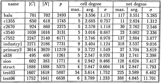
5.1 Properties of test circuits, (p is the number of pins, a is standard deviation, avg is a v e r a g e .)... ,38

5.2

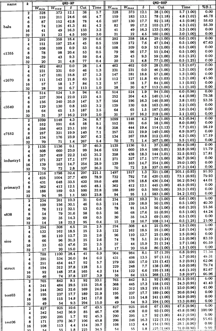
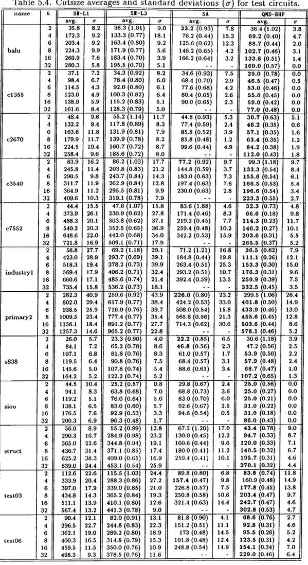
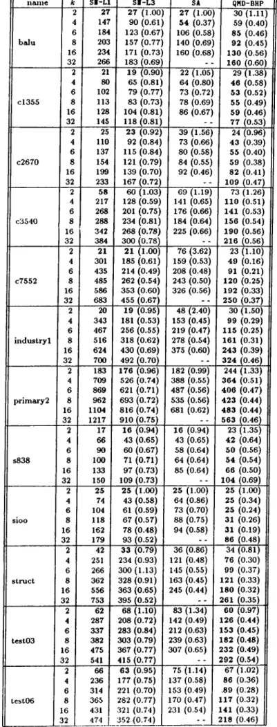
Dual Graphs of Test C ircuits... 38 5.3 Comparison of QMD-HP and QMD-BHP. {Wmai and W,nin are the

maximum and minimum part weights respectively, 8 is unbal­ ance ratio, %B.I. is the percent balance improvement in QMD-BHP.) 41 5.4 Outsize averages and standard deviations (a) for test circuits. . 42 5.5 Minimum cutsizes for benchmark circuits. (Bold values are the

best values in each r o w . ) ...

44

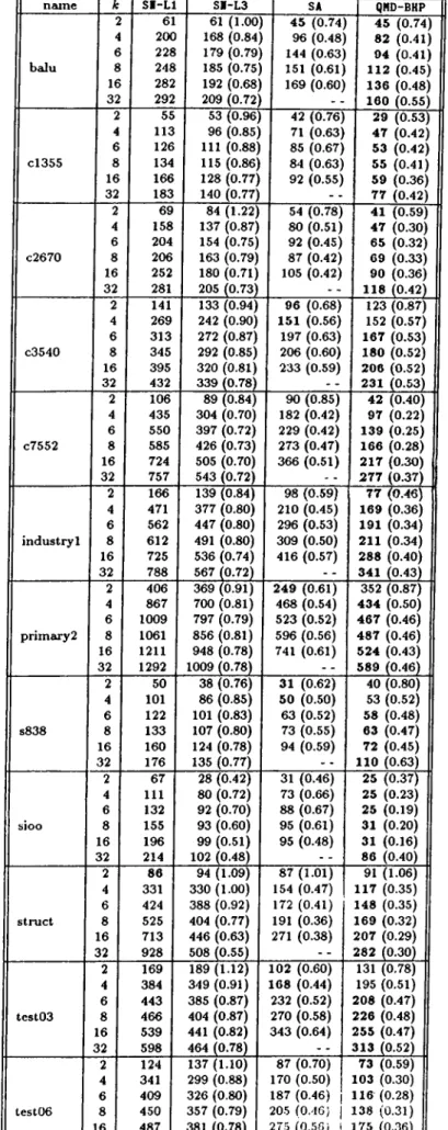
5.6 Maximum cutsizes for benchmark circuits. (Bold values are the best values in each r o w . ) ...

45

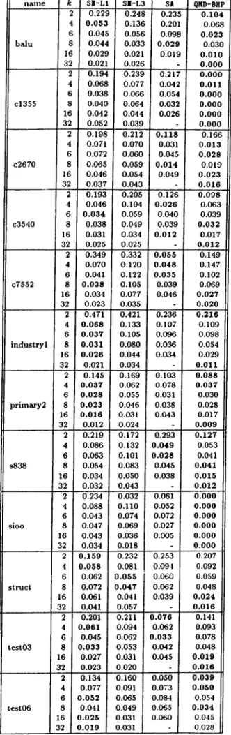
5.7 Stability Ratios (ratio of standard deviation to cutsize) for benchmark circuits.(Bold values are the best values in each row.) 46

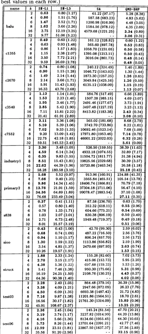
5.8

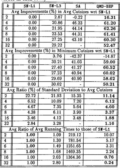
Execution times for benchmark circuits (in seconds). (Bold val­ ues are the best values in each r o w .)... 47 5.9 Average (Avg) results for performances of algorithms. Averages

were taken over all our test instances. (A: is the number of parts. Bold values are the best values in each r o w .) ... 49 5.10 Average percentage improvements of the proposed QMD-BHP al­

gorithm with respect to SN and SA algorithms for different num­ ber of parts. Averages were taken over all our test instances,

k

is the number of parts... 49

Chapter 1

Introduction

Divide and conquer strategy underlies in the solution of the hard problems. It is based on dividing the problem into small sub-problems contributing to the solution of the fundamental problem, hence this division reduces the search space. This strategy is mostly used in the combinatorial optimization problems and in VLSI layout design.

In VLSI layout design, electronic circuits are modeled as graphs (hyper­ graphs), in such a way that modules and interconnections in the circuits are represented cis nodes and edges (nets), respectively. Divide and conquer strat­ egy assists in solution of the layout design problem. The sub-problems are arised by dividing or partitioning the circuit into two or more parts by satisfy­ ing the some balance criteria. The total interconnections between these parts must also be minimized to have a better solution for the whole problem. In the literature, this partitioning problem is referred as graph/hypergraph parti­ tioning or mincut partitioning.

The graph (hypergraph) partitioning problem is NP-hard [5]. Hence, heuris­ tics giving suboptirnal solutions in polynomial time are used to solve the prob­ lem. Known heuristic algorithms can be divided into two groups;

1

. Iterative algorithms,

2

. Constructive algorithms.

Iterative algorithms start with an initial solution, and try to improve this initial one, at each iteration, until a local optima is found. One of the most

CHAPTER 1. INTRODUCTION

popular heuristic is Kernighan-Lin [13] method. It is an iterative graph bipar­ titioning heuristic, in which each iteration contains a number of cell (module)

swaps on the balanced partitions. Many of the subsequent algorithms are based on this heuristic. The same swap strategy is applied to hypergraph partitioning problem by Schweikert-Kernighan [23]. Fiduccia-Mattheyses [

4

] introduced a better data structure and cell move strategy. Their method works on unbal­ anced partitions given the lower and upper bound on the partition sizes. The time complexity of one pass (iteration) of the method is also reduced to linear in the size of circuit. Krishnamurty [17] extended the cell gain concept by introducing a look-ahead ability. However his method is also a bipartitioning method as Fiduccia-Mattheyses’ . Sanchis [22] extended this formulation to the multiple-way partitioning.

There are many other heuristic approaches such as Simulated Evolution [14] and Simulated Annealing [15]. In general, Simulated Annealing (SA) has the best solution quality among all those known heuristics. Optimization in the parameters of SA and extensive empirical studies have been done by Johnson et. al. [9].

Kahng [

11

] introduced a constructive bisection algorithm based on the in­ tersection graph G which is dual to the input hypergraph. However, his al­ gorithm produces unbalanced partitions, since no weight information is kept in the intersection graph. Kamidoi et.al. [

12

] introduced a new constructive algorithm called Weighted Hypergraph Bisection (WHB) with the notion of net- graph. WHB is an extension of Kahng’s method. It produces more balanced partitions than Kahng’s method and comparable cutsize results.

Although the treatment so far is mostly graph theoretic, motivation for the work is from the direct solution of sparse linear systems [

21

]. One phase of the direct solution is to find a new ordering for rows and columns of matrix, to reduce the fill-in in the forward and backward substitution phases, which is also a NP-hard problem [27]. Minimum Degree Ordering, proposed by Tinney[25], is the most popular heuristic algorithm. It works on the structure of the matrix, therefore it is a graph algorithm. Liu [18] shows that minimum degree ordering (MD) results in partitioning by node separator.

Proposed algorithm in this work is based on the minimum degree and dual graph of the input hypergraph. Our dual graph is similar to the intersection graph of Kahng. There is one node in the dual graph corresponding to each net

CHAPTER 1. INTRODUCTION

in the hypergraph. Two nodes in graph are connected only if the respective pair of nets have at least one cell in common in hypergraph. Given this definition node separator in the graph determines a cut in the hypergraph.

Our algorithm is based on the following well-known observation:

O bservation

1

Assigning cells (modules) to the parts to minimize the cutsize is equal to assigning nets to parts (making them internal netsj in order to maximize the number of nets that are not in the cut.

Proposed algorithm chooses a net to make internal by a heuristic based on the minimum degree ordering. However, instead of assigning the net to some part, it enlarges a cluster by adding the selected net. Therefore, it can also be considered as a clustering algorithm. We have also realized that, with a slightly different perspective, the partitioning problem can also be expressed by the clustering problem, i.e. if we allow to enlarge clusters up to a given partition size, we get a partitioning on the input. However, we may get more parts than required. As the current cut between clusters is realized, the problem is reduced to the number partitioning problem. This NP-hard problem can also be solved by a simple heuristic such as First Fit Decreasing.

The outline of the work is as follows, the next chapter gives some prelim­ inaries about the graph/hypergraph partitioning problem and more detailed information about the previous works. Minimum degree ordering algorithm which is the basis of our algorithm is explained in the third chapter. The fourth chapter discusses the proposed algorithm. Empirical studies are given in the fifth chapter and the conclusions are presented in the last chapter.

Circuit Partitioning and Previous

Works

Chapter 2

2.1

Preliminaries

Hypergraph H = ((7, N) is defined as a set of cells C and a set of nets (hyper­ edges) N between those cells. Since in VLSI, circuits are modeled as hyper­ graphs, cell set C denotes the set of modules, and net set denote the interaction between modules. Every net n, G is a subset of cells. The cells in a net are called pins or terminals of the net.

We say that cell c is incident to net n if c G n, and two cells which are incident to same net are called adjacent, in other words, cells in a net are adjacent. Degree of a cell is denoted by deg{c) and it is the number of incident nets. In general, minimum node degree is assumed to be

1

, i.e. deg{ci) >

1

for

1 < i < \C\. We use the notation \C\ as the cardinality of set C. Cells with degree zero are called as isolated cells, and they do not introduce problems in partitioning. The degree of a net is the number of pins (terminals). It is also assumed that every net contains at lerist two pins i.e. |n| >

2

.

or

In a hypergraph the total number of pins p is defined as P =

X)

¿ep(c)

cec

p = X l«l·

(

2

.

1

)

CHAPTER

2

. C m C U ir PARTITIONING AND PREVIOUS WORKS 5

Graph G = {C, E) is a special case of hypergraph such that each edge con­ tains exactly two terminals. Therefore, algorithms proposed for hypergraphs can work on graphs without modifications. Since our aim is to solve circuit partitioning problem and hypergraph models the circuit better than graphs, we will explain partitioning algorithms using hypergraph notation.

For hypergraph H = (C, A'^), the weight function on cell set maps each cell to a positive integer, i.e. for each c € G, weight{c) > 1. We can think that this function maps each cell to its area in the layout. The cost function on net set is defined in the same manner, i.e. for each n £ N, cost{n) >

1

. Definitions of

lueight and cost function can be extended for a set. Let A Q C and M C N

then

weight(A) = weight{c)

cEA

COSt{M) = ^ 2 cost{n).

tiEM

Using this notation total weight of circuit can be expressed as weight(C) and total cost of nets is cost{N).

k-way partition of hypergraph H is defined as

D efin ition 1 V = {P1 1P2·, · · · 1 ^Jt} k-way partition o f hypergraph H if and only if the following three conditions hold:

• Pi c C and Pi 0 /o r

1

< f < fc

• u L . p. = c

• P in P j = Sl f o r i < i < j < k

When it = 2 we call this partitioning as bisection or bipartition.

For a partition "P, a net n is said to be internal in partition P, if and only

Vc € n, c € Pi

if

or

The set of internal nets N[ is defined as Nj — {n|

7

i is internal net in a partition } or Nj = {7r|7Z n Pi = n ior n G N and Pi G V } and the set of external nets Ne is defined as Ne = {n|n fl P,· 0 and n H P, ^ n for n G N and P, G V }. Cut size C is defined as

C{V) = ^2 cost{n)

CllAPrER 2. CIRCUIT PARTITIONING AND PREVIOUS WORKS

6

neNE

or

C{V) = COSt{NE).

Using different expression

C{V) = cost{N) — cost{Ni).

A partitioning is balanced if all parts have about the same weight. When all parts have exactly the same weight, we call this partitioning as perfectly balanced. Note that perfect balance is not possible in ¿-way partitioning if the total cell weight is not a multiple of k.

2.2

Problem Definition

Let N be set of natural numbers. Given a hypergraph H = (C ,N ), a weight function weight : C Af, a cost function cost : N JV let Vi = {P i, P

2

, . . . , P*} be a ¿-way partition as defined in Definition

1

satis­ fying the condition

VTmaa;

l^max < A

where Wmin and W^ax are minimum and maximum partition weights, respec­ tively, and A is predetermined imbalance ratio. Also let IT = {V\.,V2·, ■ ■ ·} be

the set of all feasible solutions.

Q u estion Find a feasible solution (partition) V that minimizes the cutsize over all feasible solutions, or more formally;

m inC(P) = cost{N) — cost{Nj).

This cost definition computes each external net once regardless of the num­ ber of parts which pins of the net distributed. Other cost definitions can be done using this number, such that let I be the number of parts which a net n

CHAPTER 2. CIRCUIT PARTITIONING AND PREVIOUS WORKS

The hypergraph partitioning problem is NP-hard [

5

]. Although the graph is a special case of hypergraph in which each edge connects exactly two cells, it is also NP-hard problem. Any heuristic which solves the hypergraph partitioning problem can be used for graph partitioning problem, but graph partitioning heuristics need modifications to handle hypergraph partitioning.

Some other cost function definitions are also available in the literature. In the next section we will review the previous works on this problem in detail.

2.3

Previous Works

Available heuristic algorithms can be divided into two groups; iterative and

constructive algorithms. Although there is a substantial amount of literature on the iterative approaches, the literature that addresses the constructive algo­ rithms are rare and more recent. Now let us review the some of those heuristics:

2.3.1

Iterative Algorithms

Kernighan-Lin’s Method :

This heuristic is a graph bipartitioning algorithm [13]. It works on the balanced partitions, starts with an initial partition (mostly random) and at each iteration the cutsize is reduced by a number of cell swaps. In order to get a balanced partition after a swap, all cells must be equally weighted. This scheme is not applicable for the current problems.

Gain of a swap is calculated as a reduction in the cutsize. All swap gains are computed and the cell pair with the largest gain is selected for swap. These two cells are tentatively interchanged and they are locked in their new partition in order to prevent the algorithm falling in an infinite loop. The cell swap gains of adjacent cells are recomputed since there may be a change due to current swap. The next largest swap gain cells are selected to swap next, and this loop goes until all cells are locked to complete a pass.

At the end of each pass the maximum prefix sum of gains (which must be positive) are calculated and the cell swaps whose gains are included in this prefix sum is done. If maximum prefix sum is not positive, this means that no

CHAPTFAt 2. C m C l i r PARTITIONING AND PREVIOUS WORKS

8

further improvements can be done and algorithm terminates. If it is positive, all cells have been unlocked and algorithm starts a new pass. Maximum prefix sum strategy allows the algorithm not to stuck in a local optima.

This algorithm is a bisection algorithm but, it can be also used for k-

way partitioning using the heuristic recursively, if /: is a power of

2

. The time complexity of one pass is 0{n^ log n) where n is the number nodes in the graph. Empirical studies show that this heuristic results in poor cutsize in very sparse graphs and in special type of graphs such as ladder graphs [

1

].

Schweikert-Kernighan’s Method :

This heuristic [23], is the application of the swap strategy to hypergraph partitioning problem. Up to this work, graph model Wcis used for hypergraph partitioning problems.

Fiduccia-Mattheyses’s Method :

Fiduccia-Mattheyses (FM) [4] introduced the notion of cell move, as well as the new data structure, for the the hypergraph bisection algorithm. Cell move gain is computed as reduce in the cutsize and gains are put into bucket list.

This reduces the time complexity of sorting nodes according to their gains to linear in the number of nodes and edges. That is, let p denotes the total number of pins, which is calculated as in the Equation

2

.

1

, then the time complexity of one pass is 0{p).

Hence the cell move strategy is used in this algorithm, and this heuristic can work on unbalanced partition. Given the lower and upper bound on the size of the parts, algorithm distinguishes the feasible and infeasible moves. It starts with an initial solution and it makes a number of cell move at each iteration. Same prefix sum strategy of Kernighan-Lin’s method is also used as hill-climbing technique. Because of its ability of working on the unbalanced partition, many of the subsequent algorithms use the same balance criteria.

Krishnamurty’s Method :

This heuristic [17] is an extension of FM’s method. Look-ahead ability is added to the cell gain concept by considering the number of pins of a net in a part. Each node has a gain vector with size /, where / is the number of levels.

First level gain is same as that in FM’s method. Second level gain, shows the possible cut size reduction in the next move which follows the the current cell

CHAPTER 2. CIRCUIT PARTITIONING AND PREVIOUS WORKS

9

move. If a net has

2

cells in a part (A), and at least one cell in other part

(B ), moving one of the two cells from A to B does not reduce the cut size, but it gives the chance to the other cell of this net, to reduce the cut. Therefore effect of this net to first level gain of those cells are

0

and effect to second level gains are the cost of this net.

Sanchis’s Method :

Sanchis generalized the Krishnamurty’s method to the multiple-way (k-

way) circuit partitioning. Since there are more than one part which a cell can move, each part contains k — I bucket list; one for each other part which a node can move. Hence, k must enter the run-time complexity of the algorithm. The time complexity of one pass is 0 { l -p - k · (log k -f Gmax · 0)> where / is the number of levels and Gmax is the size of buckets.

Simulated Annealing :

Simulated Annealing starts from a randomly chosen initial configuration, the configuration space is searched for the best solution using a probabilistic hill-climbing algorithm. In order to search , the neighborhood of a configuration must be defined. Neighborhood consists of all configurations which can be obtained by moving one node from a part to another part. At each iteration, one of the possible moves is chosen as a candidate move. Then decrease in the cutsize is calculated without changing the configuration. If candidate move decrecLses the cutsize, it is realized. If it increases the cutsize, then it is realized with a probability which decreases with the amount of increase in the total cutsize. Acceptance probabilities of moves that increase the cost are controlled by a temperature parameter T which is decreased using an annealing schedule. Hence, as the annealing proceeds, acceptance probabilities of uphill moves decrease. This method over performs, in the quality of cutsize, all the previous explained Kernighan-Lin based approaches [15]. However, its run-time is to large, this makes it impractical. Optimizations in parameters of Simulated Annealing, and extensive empirical studies have been done by Johnson et. al. [9].

Ratio Cut :

Wei-Cheng [26] [2] present a new heuristic called Ratio Cut. This is ba­ sically, Kernighan-Lin based hypergraph bisection heuristic with a new cost function. They put the balance criteria into the cost definition. Their method

CHAPTER 2. CIRCUIT PARTITIONING AND PREVIOUS WORKS

10

gives highly uneven partitions. Hybrid Approaches :

It is known that Kernighan-Lin based algorithms perform poorly in very sparse graphs (hypergraphs) and in large graphs. To handle this problem a number of clustering method have been proposed. Cong-Smith [

3

] introduced a clustering algorithm which works on the graphs. They convert the hypergraph to the graph by representing a r-terminal bet by a r - clique. Then they use a heuristic algorithm to construct the clusters. The clustered graph is given as input to the Fiduccia-Mattheyses algorithm. Shin-Kin [24] proposed a clustering algorithm which works on hypergraphs, then a KL based heuristic is used to partition the clustered hypergraph.

2.3.2

Constructive Algorithms

Some of the constructive algorithms are based on eigenvector approaches such as Hadley et.al [7] and Hagen-Kahng [

8

].

As can be noticed, the clustering algorithms explained in the previous sec­ tion can also be expressed as a constructive algorithm, if we allow to enlarge a cluster up to a partition size.

Two well known constructive heuristics are : Kahng’s Method :

Kahng [11] presents a constructive hypergraph bisection algorithm which has a run-time complexity O(n^) where n is the number of nodes in the hyper­ graph. His algorithm constructs an intersection graph from the given hyper­ graph. Each node of the graph corresponds to a net in the hypergraph and two nodes in the graph are connected only if the respective pair of nets have at least one cell in common in hypergraph. Note that this intersection graph concept is similar to the dual graph concept exploited in this study (Section 4.1). His algorithm selects a seed node at random and finds the furthest node from it in the intersection graph. Then it uses breadth-first search, starting from those two nodes, to find an initial cut in the intersection graph. This initial cut in the intersection graph corresponds to a partial bipartition in the hypergraph. The partial bipartition is completed by a PLA folding based algorithm resulting in

a bipartition of the hypergraph. This method gives uneven partitions, since no size information is stored in the intersection graph.

W H B :

Kamidoi et.al. [

12

] extend the Kahng’s method, by introducing the net- graph where nets are also taken as nodes in addition to the cells of the hy­ pergraph. The edge set of the netgraph contains the incidence information of the hypergraph. That is, if a cell in the hypergraph is incident to a net, then the corresponding cell-node in the netgraph is adjacent to the corresponding net-node. Their algorithm selects a random net-node as a seed and finds the furthest net-node to use as the second seed. Modified version of breadth-first search is then used to construct an initial cut. It takes care of the weight of the parts. Then, a heuristic is used to complete the cut into a bipartition of the hypergraph. Their algorithm also requires 0{n^) computation time. Their cutsize results are comparable with the Kahng’s method. Their test data were sparse and random and they claim that algorithm WHB performs 14% better than FM.

Chapter 3

Minimum Degree Ordering

The motivation for this work is from the direct solution of large sparse linear systems. Let A be a large n-by-n sparse symmetric positive definite matrix. The direct solution of the linear system

A x = b

involves factoring the matrix A into LL^, where L is the lower triangular Cholesky factor of A . When A is factored, it normally suffers some fill. Since P A P ^ is also symmetric and positive definite for any permutation matrix P , we can instead solve the reordered system

(P A P '^ )(P x ) = P b.

The choice of P can have a dramatic effect on the amount of fill that occurs during the factorization. Thus, it is standard practice to reorder the rows and columns of the matrix before performing the factorization.

The problem of finding a best ordering for A in the sense of minimizing the fill is computationally intractable: an NP-hard problem [27]. We are, therefore, obliged to rely on heuristic algorithms. By far, the most popular fill- reducing scheme used is the Tinney’s Minimum Degree (MD) algorithm [2.5], which corresponds to the Markowitz scheme [20] for unsymmetric matrices. This scheme is based on the following observation;

Suppose that ¿ — 1 rows/columns are selected for reordering. Note that this corresponds to determining the first ¿ —

1

rows/columns of the P matrix. The number of non-zeros in the filled graph for those rows/columns is fixed. In order to reduce the number of non-zeros in the ¿-th row/column, it is intuitive

CHAPTER 3. MINIMUM DEGREE ORDERING

₁₃

that in the sub-matrix remaining to be factored, the row/column with the fewest non-zeros should be selected as the i-th row/column. In other words, the scheme may be regarded as a method that reduces the fill of a matrix by a local minimization.

3.1 The Basic Algorithm

The MD algorithm can easily be described in terms of ordering a symmetric graph using the elimination graph model [

21

]. Generally, it works only with the zero/nonzero structure of a symmetric matrix and simulates in some manner the steps of symmetric Gaussian elimination. The zero/nonzero structure of a sparse symmetric matrix A can easily be represented by a structure graph Each row/column i in a sparse matrix A is associated with a node i in its structure graph. Two nodes i and j in the structure graph are connected (i.e., { i , j } € only if 0 in the sparse matrix A . Let

Go = (Vb, Eo) = G^ be the structure graph of given matrix. We will use notation Gi to denote the z-th elimination graph which is obtained by the elimination of i nodes from the initial graph Go. adjo-{x) denotes the adjacency list of the node x in the z-th elimination graph Gj. At each elimination step a node Xi in G,_i is selected, and eliminated graph Gi is obtained from G,_i by:

• deleting node x,· and its incident edges in G,_i,

• adding edges to graph so that nodes in adja^_^{xi) are pairwise adjacent in Gi.

Based on the transformation rule, we note that if a node v is not adjacent to Xi in G,_i

adjoiiv) = adjoi^iiv)

However, if u G adjoi-i (xi), then we have

iidjaM') = {(idjG^-x[^i)0 adjG,_,[v)) - {u,x,·}.

Therefore, only the degree of a node in adjGi_t{xi) may change after the elim­ ination graph transformation from G,_i to G, due to the deletion of edges incident to Xi and possible addition of new edges joining nodes adjacent to

CHAPTER 3. MINIMUM DEGREE ORDERING ₁₄

F u n ction MinitmimDegree Go <-

i ^

1

w h ile I < |F^| do

In the elimination graph (7,_i = (K _ i,F ,--i), choose a node X{ of minimum degree Form the new elimination graph G{ = (VJ, F,),

by eliminating the node from G,_i f f +

1

en d F u n ction

Figure 3.1. Basic Minimum Degree Algorithm

Xi. Using the elimination graph model, the basic algorithm is presented in Figure 3.1.

Filled graph of G"^ = is defined ¿is symmetric graph G^ =

E^), where F = L + L^. Obviously, and E^ consists of all edges in and all filled edges during factorization. The filled graph G^

can easily be constructed from the sequence of elimination graphs using the following lemma.

L em m a 3.1 The edge {xi^Xj] G E^ if and only if {xi,X j} ^ E or G

E^ and G E^ for some k < m in {f,;}.

3.2

Implementation with Quotient Graph Model

The characterizations of G, (for i =

1

, . . . , |U'^|) and E^ can be directly com­ puted in terms of the original graph G"^, using the reachable set concept. Let

5

be a subset of the node set and u ^ S. The node u is said to be reachable

from a node y through S if there exist a path (y, Ui,. . . , ut, u) from y to u for

k > 0 such that u, G 5 for 1 < i < /:. Reach{y, S) denotes the reachable set of y through 5, and defined as

CHAPTER 3. h'llNlMUM DEGREE ORDERING

₁₅

The edge set of the elimination graphs can be computed using the following theorem

T h e o r e m 3.1 [6] The edge { u, u} e Ei if and only if v e Reach{u,Si), where Si = { i i , . . . ,a:,·} denotes the sequence of nodes eliminated in the first i steps of the MD algorithm.

Hence, the adjacency set of a node u ^ Si in G, can be calculated by generating the reachable set of u through Si., i.e.,

adjofu) = Reachooiu, S i) fo r i = 1 , . . . ,

The only disadvantage of this implicit representation is the amount of work required to determine reachable sets can be large, especially at later stages of elimination. However, it has a small and predictable storage requirement. Note that the maximum amount of storage requirement is unpredictable in the explicit representation of elimination.

The quotient graph concept is introduced to reduce the amount of work to generate reachable sets. In quotient graphs, connected eliminated nodes are coalesced in order to shorten the length of paths to uneliminated nodes. Let G = (V, £■) be a given graph and let P be a p-way partition on its node set V:

V = ( V „ ...,V ,)

That is Ufc=i Vk = y a^nd K H Lj = 0 for i

7

^ j. We define the quotient graph of G with respect to V to be the graph G /P = (V ,S ), where {K , Vj) E € and only if adj{Vi)

n

Vj

7

^ 0. Here, adj{Vi) = UveK «4?g(v)·

D efin ition

2

Let V (S ) denotes the set of connected components in the sub­ graph G{S).Then the partitioning on the node set V,

V{S) = V iS )0 {V - S) uniquely defines the quotient graph GjV{S).

Hence, elimination graphs can be efficiently represented using quotient graphs according to the following theorem:

CHAPTER 3. MINIMUM DEGREE ORDERING

₁₆

Theorem 3.2 [6] For v ^ V — Si,

Reacho{v,Si) = ReacliQ^{v.V{Si)) where

Qi

= G '/V (5.) = (V (5,),i.·).

Chapter 4

Circuit Partitioning Using M D

Ordering

The algorithm presented in this work is based on the MD ordering algorithm. Our algorithm uses quotient graph model for elimination, because of its storage advantage over the basic MD algorithm. Quotient graph model basically inher­ its the storage advantage of reachable sets model, and improves the run-time of this model by introducing supernode concept which is not more than coalescing the connected eliminated nodes. The proposed algorithm will be referred here as Quotient Minimum Degree for Balanced Hypergraph Partitioning (QMD-BHP) algorithm.

Section 4.1 presents the dual graph concept. The idea behind the node selection scheme in the dual graph and its correspondence to the original hy­ pergraph are discussed in Section 4.2. Algorithms for size and valence com­ putations needed in node selections are presented in Section 4.3. Section 4.4 contains discussion about the elimination graph transformations to be per­ formed after node selections. An algorithm to improve the balance quality of the partition found by the QMD-HP algorithm is proposed and presented in Section 4.5. Finally, Section 4.6 discusses the computational complexity of the proposed QMD-BHP.

CHAPTER 4. CIRCUIT PARTITIONING USING

A/D

ORDERING

₁₈

4.1

Dual Graph

Let hypergraph H = (C, N) be given where C is set the of cells, and N is the set of nets (hyperedges). Each n ^ N is a. subset of C which has a cardinality of at least two, i.e. each net connects two or more cells. There is one node in

G corresponding to each net in H. Two nodes in G are connected if only if the respective pair of nets have at least one cell (pin) in common in H. Let pins{n)

denotes the set of the cells incident to net n, and nets{c) denotes the set of the nets connected to cell c. Subscript H and G will be used to denote hypergraph and graph, respectively. For example, pinsnin) will denote the pin-list of net

n in hypergraph H, and pinsa(n) will denote the pin-list of the net associated with the node n in graph G. As will be explained later, pinsoin) is a dynamic

li.st, whereas pins}{{n) is a static list. We will skip subscript if it is clear from the context. Using this notation, formal definition of dual graph is as follows;

D efin ition 3 Dual graph of hypergraph H = (C, N) is a graph G = (W, E), where N, net list o f H , is the node set of G, and e = {n ,, n j} G E if and only if m ,nj G N, for 1 < i , j < |/V|, such that i / j and pinsnirii) fl pinsninj) ^

0

.

Our dual graph has several attributes cissociated with each node. The attributes pinso{n) and onepinsfn) for each node n oi G are defined as follows

• onepins{n) = {c|c G pinsnin) and degn{c) — 1}. • pinso{n) = pinsf{{n) — onepins(n).

A cell is called a one-pin cell if its degree is one, i.e. it is connected to only one net in H. Note that only one-pin cells in H do not introduce any edges into G. Hence, these cells are excluded from the pin-lists of the respective nodes in G. One-pin cells connected to net n is denoted by onepins{n). Hence,

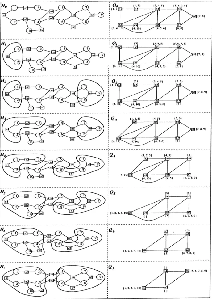
\pinsH{n)\ = |pmsG(n)| + \onepins{n)\. Figure 4.1 illustrates a sample hyper­ graph H with 10 cells, 9 nets and its dual graph G with 9 nodes, 15 edges. The pin-lists of the nodes of the dual graph are illustrated in brackets. In this example, pinsnins) = { 7, 8, 9} whereas pinsoiris) = { 7, 8} since cell 9 is a one-pin cell and hence onepins{ns) = {9}.

By referring to Definition 2, Q = G /^ {S ) = (]^{S),S) denotes the dual quotient graph of hypergraph H. Hence, Q, = (W{Si),£i) corresponds to

CHAFTER 4. CIRCUIT PARTITIONING USING MD ORDERING

19

the ¿-th elimination graph G{ =- (Ni^Ei) where 5,· = { n i , . . . , n,·} is the se­ quence of ehnunaUid nodes in the first i steps of the MD algorithm. Fig­ ure 4.2 illustrates the pseudo-code for the dual graph construction algorithm. In this pseudo-code, attributes without subscript refer to the dual graph do­ main. Here, adjQ{n) refers to the set of nodes adjacent to node n in Q, and

degQ{n) refers to the number of nodes in this set, i.e. degQ{n) = |ac(?(

2

(n)|. Note that = N, and hence Q o = G o initially. First outer for-loop in Figure 4.2, initializes the attributes of nodes of Q. Second outer for-loop con­ structs the edge set € oi Q and computes onepins attribute and initializes the pin-list of each node. Third outer for-loop initializes other node attributes to be used for node selection during the QMD algorithm.

4.2

Node Selection

We will discuss here only the partitioning of hypergraphs with unweighted cells and nets for the sake of clarity of the presentation. The proposed algorithm is applicable for hypergraphs with weighted cells and nets with minor modifica­ tions. In partitioning of a hypergraph with unweighted nets, the cutsize C{V)

CHAPTER 4. CIRCUIT PARTITIONING USING MD ORDERING

₂₀

/* input : a hypergraph H = ((7, N) *f

/* output : a dual quotient graph Qq = */

Function ConstructDual{H, Q) e ^ 0 for n = 1 to |A^| do pins{n) <— 0 onepins{n) <— 0 for c = 1 to \C\ do if dcgnic) = 1 then

let n be the only net incident to cell c (i.e. netsjq{c) = {n })

onepins{n) <r- onepins{n) U {c}

else

for each n € netsnic) do

pins{n) <— pins{n) U {c }

for each net pair {n,-,nj} incident to cell c (i.e. 7?.,-,nj € netsuic)) do

S S (J {{n .-,n j}}

for n = 1 to |A^| do

csize(n) |prniii/(n)|

valence{n) *— degQ{n)

for each m G adjQ{n) do

if {pins{m) C pins{n)) and {onepins{m) = 0) then

valence(n) +— valence{n) — 1

endFunction

CHAPTER 4. CIRCUIT PARTITIONING USING MD ORDERING 21

of a partition V simplifies into

C{V) = |7V£:| = |.V| - |.V/|.

Hence, min-cut hypergraph partitioning becomes equivalent to maximizing the number |A^/| of internal nets. In the proposed algorithm, selecting a node n in G corresponds to making net n in H an internal net. Initially, in Go = <j, all nodes are assumed to be separator nodes and there exists no node-clusters.

Hence, in i/o, all nets are assumed to be external nets and there exists no

cell-clusters.

Consider selecting a node n, in the elimination quotient graph Q ,_i. If there exists no previously selected node in the adjacency list of n,·, node n, becomes a cluster node n, in Q, representing the node-cluster A^„, in G,. Otherwise, node

Hi combines with the cluster nodes in its adjacency list to become a cluster node in Qi representing the node-cluster

Wn. =

U

I U {n,}

(4.1)

in G,, where cadjQ-_^{ni) = D adjQ._^{rii) represents the set of cluster nodes adjacent to n,· in Qi-i. Recall that 5,_i = { u i , . . . n ,_ i} denotes the sequence of nodes selected during the first t — 1 steps, and Af{Si-i) denotes the overall set of cluster nodes in Qi-i. Note that cluster nodes in cadjQ^_^{ni) are removed from the cluster node set Af{Si) during this transformation. In both cases, the new node-cluster in G, induces a new cell-cluster G„. in Hi. In the former case, the respective cell-cluster G„, in Hi contains only the pins of n,·, i.e. pinsf{{Cni) — pinsfj{ni). In the latter case, pins of net n, combine with the pins of the cell-clusters in H corresponding to the cluster nodes in cadjq._^

to form a new cell-cluster Cm- That is,

p i n s H { C m ) = \

U

plnsjj{Cn,)\

u

pinsnirii)

{4.2)

In this notation, each cell-cluster in H is labeled with the last net made internal in that cluster. Note that node-clusters and the respective cell-clusters consti­ tute connected components in G and i / , respectively. Figure 4.3 illustrates the elimination steps in the dual quotient graph of the sample hypergraph given in Figure 4.1. In this figure, each Qi is also associated with the respective Hi

to illustrate the cell-cluster formation. Selection of in Qi which forms the cell-cluster G„g, where pinsniCm) = pinsnins) = {7 ,8 } is an example for the

CHAPTER 4. CIRCUIT PARTTTIONINC USING MD ORDERING

22

former case. Selection of nr in Q3 which form the cell-cluster Cm such that

pinsff{Cm) — pinsf{{Cng) 0 pinsfi(nr) = {6 ,7 ,8 ,9 }, where ns 6 cadjQ^(nr), is

an example for the latter case.

Consider the selection of a node n, with the minimum degree in the elimina­ tion graph Gi-i to form a node-cluster in G,. This choice is a greedy choice in the hope that nodes with smaller degree will introduce less fills compared to the nodes with larger degrees. However, if the node-cluster satisfies l-^nj + \0'djG{Nm)\ < |A^|, o,dja{Nni) forms a separator for Nm- Furthermore,

we have

T h e o r e m 4.1 [19j adja^mini) = adjoiNm) and de^fG..,(n,·) = |ad;G(A^n,)|·

Hence, the greedy choice in selecting node in G,_i also corresponds to a locally optimal choice in minimizing the node-separator size |ad;G(-/Vn, )|. Note that nodes in adja{Nm) will either combine with cluster to form new clusters or remain in the separator during the future node selections. In other words, they have no chance to be included in other node-clusters which will not contain Nm · Hence, local minimization of the separator size also has the desirable effect of even distribution of the remaining unselected nodes among the other node-clusters.

In the proposed algorithm, we grow node-/cell- clusters in GIH as connected-components similar to MD algorithm. However, the criteria for se­ lecting a node n,· in G,_i is the local minimization of the net-cut (net-separator)

size of the cell-cluster Cm that will be induced by the node-cluster Nm to be formed upon selecting n,·. Let,

extnetsfj(Cn,) = {^j € N | pinsn(nj) D ^ 0

A pinsninj) - pinsH(Cm) (4.3) represents the set of external nets (real net-cut) of cluster G„,. That is, an external net of a cell-cluster has at least one pin in that cluster and at least one pin outside that cluster. In a dual analogy to the MD algorithm, nets in extnetsH(Cn,) will either become the internal nets of the cluster that will contain Cm or remain in the net-cut in the future node/net selections in G /H.

That is, they have no chance of becoming internal nets of cell-clusters which do not contain Cm- Hence, similar to the MD algorithm, local minimization of the net-cut size also has the desirable effect of even distribution of the remaining unselected nets as internal nets among the other cell-clusters.

CHAPTER 4. CIRCUIT PARTITIONING USING MD ORDERING

23

CHAPTER 4. CIRCUIT PARTITIONING USING MD ORDERING

₂₄

The net-cut size of a cell-cluster that will be induced by the node-cluster to be formed upon selecting a node in G will be referred here as the valence of that node. However, large number of ties occur during node selections according to the valence values as in the MD algorithm. The selection of the next node with minimum valence from the candidate set is effectively determined by the initial ordering which essentially determines the way ties are resolved. In this work, we propose a tie-breaking strategy which enables growing balanced cell- clusters. In the proposed algorithm, when more than one node has the the same valence, the one with the minimum cluster size is selected first. Here, cluster size of a node in an elimination graph refers to the size of cell-cluster that will be induced by the node-cluster to be formed upon selecting that node. If the cells of the hypergraph are unweighted, the size of a cell-cluster is equal to the number of cells in that cluster. Our selection scheme does not allow a cluster to grow beyond a predetermined maximum part size. That is, unselected nodes whose cluster sizes exceed the indicated maximum part size are not considered during selections. The maximum part size is selected as ^ · (1 + j ) where A is the imbalance ratio (Section 2.2) and ^ denotes the size of a part under perfect balance conditions.

4.3

Size and Valence and Calculations

Both stopping criteria for cluster expansion and tie-breaking criteria necessitate the cluster size (csize) computation for each unselected node. Here, csize{n)

of an unselected node n in Qi denotes the size of the cell-cluster (7„ to be induced upon selecting n. The csizeai(n) attribute of an unselected node n in Gi can be computed by finding the cardinality of the pin-set in the right- hand side of Equation 4.2. Note that pin-sets of all cell-clusters induced by the cluster nodes in cadjQ^{n) are disjoint sets. Hence, the cardinality of the pin-set represented with first set-union operation can easily be computed by a simple addition. However, net n shares at least one pin with each cell-cluster induced by the cluster nodes. Hence, all we need to compute is the number of new pins to be introduced by net n to the cell-cluster C„. For the sake of efficiency of these computations, we maintain a dynamic pin-list {pinsa^{n) = pinsQ-{n))

for each unselected node n. Upon selecting a node n,· in Q ,-i, pin-list of each

unselected node n G updated as

CHAPrER 4. CIRCUIT PARlTriONING USING MD ORDERING

25

where nadjQ-_^{ni) = adjQ-_i{ni) — cadjQ^_^{ni) denotes the set of unselected nodes adjacent to n, in Q i-i. Hence, pinsQ^_^{n) denotes the subset of pins of net n (excluding those in onepins{n)) which are not assigned to any cell-cluster in H i-i. Thus, csizeQ-{n) of an unselected node can efficiently be computed as

csizeQ^(n) = ^ csizeQ-(tn) -f |pm5Q;(n)| -f |onepms(n)|. (4.5)

m^cadjQ· (n)

Initial computation of csize{n) is given in the last for-loop of Figure 4.2. Note that cadj set of each node is initially empty since there is no selected nodes yet. Therefore initial csize values contains the number of pins of the respective net. Upon selecting n,· in Q ,_i, the cluster size of only those nodes in rchsetQ^_^{ni)

should be recomputed for Q,·. Pseudo-code of size calculation is given in Fig­ ure 4.7. Maintaining dynamic pin-list for each node has other merits during valence computation as will be discussed later.

The node separator adja{Nm) of the node-cluster Nm in G, formed upon selecting node n,· in Gi-i already induces a net-cut (cut-separator) for the cell- cluster Cm in H. However, this induced net-cut may be an overestimation for the real net-cut of Cm in H. That is,

extnetsHiCm) Q. adjaiNm)· (4.6)

Some of the unselected nets may directly become an internal net of the cell- cluster Cm upon selecting node n, in G,. This happens for an unselected node rij € adjoiini) whenever pinsfj{Cm) 2 pinsfj{nj). We will refer to such nodes/nets as mass-elimination nodes/nets and define the mass-elimination node/net set of an uneliminated node n as

masselim(n) = adjaiNn) — extnetSf{{Cn)· (4-7) Nodes in the mass-elimination set of a node n can be eliminated together and included into Nn upon selecting n. Our implementation forces them to be selected following the selection of n. Note that they do not introduce any extra pins to the respective cell-cluster G„ in contrast to the standard node selections. Hence, the valence of a node n in the elimination graph Q, can be computed as

valenceQ^n) — degQ.{n) - |masse/fm(

2

.(n)|. (4.8) Here, degQi(n) denotes the degree of node n in Qi which is the selection criteria in the original MD algorithm. Hence, valence computations necessitate finding the mass-elimination node set for each unselected node.

CHAPTER 4. CIRCUIT PARTITIONING USING MI) ORDERING

₂₆

F u n ction ReachSet{n) rchset <— 0

fo r each v € adj(n) d o

if deg{v) > 0 th en /* v is an uneliminated node */ rchset <— rchset U {u }

else /* u is a cluster node * j

fo r each u 6 adj{v) — {n } d o

rchset rchset U { « } re tu rn rchset

e n d F u n ctio n

Figure 4.4. Reachable set calculation

T h e o r e m 4.2 An unselected node m G masselimQ-{n) if and only if onepins{m) = 0 and cadjQfm) C cadjQfn) and

either (i) m G nadjQ.{n) A pinsQ-{m) C pinsQ^n) or (ii) m G rchsetqXu) Am ^ nadjQfn) ApinsQ^m) = 0

Proof easily follows by noting the two facts. First, unassigned pins (cells) of node m should be assigned to by the selection of node n. Second, the cell- clusters which contains the previously assigned pins of m, should be merged into Cn by the selection of node n.

The third for-loop in Figure 4.2 performs the initial valence computations. The second for-loop in Figure 4.7 performs the valence update for a node which is in the reachable set of the selected node. Note that, during the Q,_i —> Q,· transformation, only the degree and mass-elimination node set of a node in the reachable set of node n, should be considered for update (See pseudo-code in Figure 4.5 and 4.7).

4.4

Graph Transformation

Let Hi be the eliminated node in the G,_i —> G, transformation and 5, = { n i , . . . , n , } be the sequence of the eliminated nodes. Recall that, at any step i of the algorithm, the node set AT(5',_i) of Q,_i contains two types of

CHAFTER 4. CIRCUIT PARTITIONING USING Ml) ORDERING

₂₇

F u n ction DegreeUpdate{rchset) fo r each v € rchset d o vrchset *— ReachSet{v) deg{v) <— \vrchset\ en d F u n ction

Figure 4.5. Degree update

F u n ction ClusterAdj{n) cadj <— 0 fo r each v € adj(n) d o if deg{v) < 0 then cadj <— cadj U {u } retu rn cadj en d F u n ction

Figure 4.6. Algorithm for finding the cluster adjacency

F u n ction UpdateVatenceAndSize(v) vrchset <— ReachSet(i')

vcadj <— Cluster Adj (v) csize(v) 0

fo r each «: ^ vcadj d o

csize{v) ·<“ csize(v) + csize{u )

csize(v) <— csize(v) + |pin.s(u)S -f ¡onepins(t valence(v) deg{v)

fo r each u € vrchset d o

if (onepins(u) = 0) and (pins{u) — pins{v) = 0) then

ucadj <— C luster Adj (u)

if ucadj C Dead;then

valence{v) <— valence{y) — 1 en d F u n ction

CHAPTER 4. CIRCVIT PARTITIONING USING MD ORDERING

28

nodes; cluster nodes and uneliminated nodes denoted by the sets A i{Si-i) and

N - S i-1, respectively. Furthermore, the edge set 6i-i contains two types of edges; edges between uneliminated node pairs and edges between cluster nodes and uneliminated nodes. Hence, given Q,_i = {W {S i-i),6i-i) with

Qo = Go, the corresponding quotient graph transformation Q,_i —> Q, can be performed as follows: cluster nodes in cadj<

2

,_, (n.) are removed from the connected component set and the cluster node n, is added as a new connected component. That is.

Ai{Si) = Ai(Si-i) - cadjQ._^{ni) U {n,·} (4.9) and n, is removed from the uneliminated node set. Recall that A/’(S',) denotes the set of connected components in the subgraph G{Si) and W{Si) = Af(Si) U

{N — Si) represents the node set of Q,. Note that, node cluster Nm in Gi is represented with the cluster node n, in Q,.

All uneliminated nodes in the node adjacency list of the cluster node in

cadjQ^_,{ni) are connected to n,· if they were not in the set nadjQ^_,{rii) U {n,·}. All edges incident to cluster nodes in cadjQ._^{rii) are removed from the edge set. That is,

Ei = Ei-i u | {n /,n ,}| n /e (nad;Q;_j(nfc) - {n,·}) where Uk e cadjQ^_^{ni)^ - {{nk,ni}\nk e cadjQ._^{rii) and ni e nadjQ._^{nk)] (4.10)

The quotient graph representation enables the use of the edge slots of the nodes in cadj{ni) for new edges to be added to the adjacency list of n,·. It is guaranteed that the number of such edge slots are larger than or equal to the number of edges to be added to the adjacency list of n, during transformation [6]. Figure 4.8 illustrates the pseudo-code for quotient graph transformation where n denotes the selected node.

4.5

More About Balancing

Although the tie-breaking strategy of QMD-BHP enables growing balanced cell- clusters, there is no bound on the minimum cluster size when the algorithm terminates. That is, when the algorithm terminates, it is guaranteed that there will be no cluster whose size exceed the maximum part size, but the partition can still be infeasible according to the problem definition (Section 2.2). The

CHAPTER 4. CIRCUIT PARTITIONING USING MD ORDERING

₂₉

F u n ction GraphTrans{n, rchset, cadj) adj[n) <— rchset

fo r each v € rchset d o

adj(v) <— (adj{v) — cadj) U {n } en d F u n ctio n

Figure 4.8. Quotient graph transformation

nice property of the algorithm is that the unselected nodes in the dual graph already induce cut-nets in the hypergraph. If those cut-nets are realized, the problem reduces to the ¿-way number partitioning problem on the sizes of cell- clusters and remaining unassigned unit-sized pins (cells) of the cut-nets. This

NP-hard problem can also be solved by a well-known heuristic namely Fii'st Fit Decreasing (FFD). Note that the number of unselected nodes/nets is an overestimation for the real cutsize. Due to the assignment of FFD, the real cutsize can be smaller than the number o f unselected nodes/nets.

Although FFD is a successful heuristic the resulting partition can also be infeasible. That is, the imbalance ratio of the resulting partition can be larger than the predetermined imbalance ratio (A ). In order to get a smaller imbal­ ance ratio, some of the cells which are assigned to the part with maximum size should be assigned to part with the minimum size, or parts should be re­ arranged, such that; the difference between the part with maximum size and part with minimum size is reduced. However, this process can increase the cut- size. We propose a simple heuristic using the cutsize overestimation property of the algorithm. We break the largest cluster into its components by making its representative node/net unselected. Recall that the representative net of a cell-cluster is the last net which was made internal to that cluster. Making a node/net unselected corresponds to breaking the respective cell-cluster into the cell-clusters whose representative nodes were adjacent to that node in the dual quotient graph during its selection. Hence, this provides more clusters with smaller sizes to FFD by introducing only one net to the net-cut. Recall that the number of unselected nodes in the dual graph is an upper case bound on the cutsize at any step of the algorithm. The selection of the cell-cluster for breakdown is greedy. The heuristic chooses the largest cell-cluster hoping that it contains more sub-clusters than a cell-cluster with a smaller size. Only one breakdown cannot be sufficient to get a feasible partition. Therefore, this