THE REPUBLIC OF TURKEY
BAHCESEHIR UNIVERSITY
FINE-TUNING CONVOLUTIONAL NEURAL
NETWORKS FOR MARITIME VESSEL
CLASSIFICATION, VERIFICATION AND
RECOGNITION
Master’s ThesisTHE REPUBLIC OF TURKEY
BAHCESEHIR UNIVERSITY
GRADUATE SCHOOL OF NATURAL AND APPLIED SCIENCE
COMPUTER ENGINEERING
FINE-TUNING CONVOLUTIONAL NEURAL
NETWORKS FOR MARITIME VESSEL
CLASSIFICATION, VERIFICATION AND
RECOGNITION
Master’s ThesisC. DENİZ GÜRKAYNAK
Supervisor: Prof. NAFİZ ARICA
THE REPUBLIC OF TURKEY BAHCESEHIR UNIVERSITY
GRADUATE SCHOOL OF NATURAL AND APPLIED SCIENCES COMPUTER ENGINEERING
Name of the thesis: Fine-tuning Convolutional Neural Networks for Maritime Vessel Classification, Verification and Recognition
Name/Last Name of the Student: Cahit Deniz GÜRKAYNAK Date of the Defense of Thesis: 06.06.2018
The thesis has been approved by the Graduate School of Natural and Applied Sciences.
Asst. Prof. Yücel Batu SALMAN Graduate School Director
Signature
I certify that this thesis meets all the requirements as a thesis for the degree of Master of Sciences.
Asst. Prof. Tarkan AYDIN Program Coordinator
Signature
This is to certify that we have read this thesis and we find it fully adequate in scope, quality and content, as a thesis for the degree of Master of Sciences.
Examining Committee Members Signature____
Thesis Supervisor ---
Prof. Nafiz ARICA
Member ---
Prof. Erkan KORKMAZ
Member ---
ACKNOWLEDGEMENTS
First of all, I would like to thank my advisor Prof. Nafiz ARICA, who is an invaluable person in the field of artificial intelligence. Without his excellent guidance and support, this project would not have been possible. I also wish to thank my dear friend Joe for his intuitive contributions to this work. Besides that, I am very grateful to my family and all my friends, who have patiently provided me through moral and emotional support in my life.
ABSTRACT
FINE-TUNING CONVOLUTIONAL NEURAL NETWORKS FOR MARITIME VESSEL CLASSIFICATION, VERIFICATION AND RECOGNITION
C. Deniz Gürkaynak Computer Engineering
Thesis Supervisor: Prof. Nafiz ARICA May 2018, 47 Pages
Autonomous maritime vessel surveillance systems have enormous implications to national defense and global supply chain. Therefore, ship detection and classification problems have been widely studied for a long time. Most of the studies have used satellite imagery, the real-time satellite imaging access is not public and image resolutions is insufficient for high-quality classification and recognition systems. As an alternative approach, consumer-level surveillance cameras have attracted great attention recently due to its cost-effectiveness and easy installation process.
Recently, deep learning has become the state-of-the-art method in computer vision field. Deep network architectures have emerged by surpassing human-level accuracy on image classification problems. Many old but powerful ideas have been revised and applied to these networks in various computer vision problems. However, the applications of deep learning methods in the analysis of maritime vessel images are limited in the literature. In this thesis, we employ the state-of-the-art deep network architectures for maritime vessel classification, verification and recognition problems. In the experiments, the most popular three convolutional neural network architectures; AlexNet, VGGNet and ResNet are used. MARVEL dataset is utilized for benchmark purposes, which contains 2M ship images. Since these networks are very difficult to train and they require lots of training samples, we follow transfer learning approach. The main contribution of this thesis is the implementation, tuning and evaluation of specific applications for maritime vessels domain. For classification task, we conduct experiments on different transfer learning techniques and we investigate their performance by transferring the weights layer by layer. We reach the state-of-the-art results by fine-tuning VGG-16 architecture. For both verification and recognition tasks, we use triplet loss heavily inspired by recent advances in the field of face verification and recognition. We achieve closely comparable state-of-the-art results on MARVEL’s both verification and recognition benchmarks.
Keywords: Convolutional Neural Networks, Transfer Learning, MARVEL, Ship
ÖZET
EVRİŞİMLİ SİNİR AĞLARINDA EĞİTİM TRANSFERİ İLE GEMİ SINIFLANDIRMA, DOĞRULAMA VE TANIMA
C. Deniz Gürkaynak Bilgisayar Mühendisliği
Tez Danışmanı: Prof. Dr. Nafiz ARICA Mayıs 2018, 47 Sayfa
Otonom denizcilik gözetleme sistemleri milli güvenlik ve küresel ticaret zinciri alanlarında büyük önem taşımaktadır. Bu yüzden gemi sınıflandırma ve tanıma problemleri üzerine oldukça uzun zamandır çalışılmaktadır. Bu konudaki çoğu araştırma uydu görüntüleri üzerine yapılmış, fakat uydu görüntüleme sistemleri herkesin kullanımına açık değildir ve çözünürlükleri yüksek kalite sınıflandırma ve tanıma yapmak için yetersiz kalmaktadır. Buna çözüm olarak son zamanlarda standart güvenlik kameraları uygun maliyetleri ve kolay kurulumları ile dikkat çekmektedir.
Derin öğrenme son yıllarda çok hızlı ilerlemeler katederek bilgisayarlı görü alanındaki en gelişmiş teknik haline gelmiştir. İmge sınıflandırma problemlerinde insan seviyesinden daha iyi başarım gösteren derin mimariler ortaya çıkmış, yapay zeka alanında uzun zamandır var olan fikirler bu mimarilere bazı bilgisayarlı görü problemleri için adapte edilmeye başlanmıştır. Fakat literatürdeki gemi imgelerinin analizi konusunda derin öğrenme uygulamaları sınırlı kalmaktadır. Bu tez kapsamında; gemi sınıflandırma, doğrulama ve tanıma görevleri için derin öğrenme alanındaki en gelişmiş teknikler kullanılacaktır.
Deneylerde, literatürdeki en popüler üç evrişimli sinir ağı olan AlexNet, VGGNet ve ResNet mimarileri kullanılmıştır. Eğitim ve test için 2 milyondan daha fazla gemi imgesi barındıran MARVEL veri setinden yararlanılmıştır. Ayrıca elde edilen sonuçların karşılaştırılması için de aynı makale referans olarak alınacaktır. Bu derin mimarilerin eğitimi oldukça zor olup, çok büyük eğitim setlerine ihtiyaç duymaktadır. O yüzden bu tezde eğitim transferi yaklaşımı uygulanmıştır. Bu tezde literatüre katkı olarak; gemi imge analizi için derin öğrenme teknikleri kullanarak sistemler gerçeklenmiş, ince ayarları ve performans analizleri yapılmıştır. Gemi sınıflandırma problemi için değişik eğitim transferi teknikleri üzerine deneyler yapılmış ve bu teknikler katman katman uygulanarak performansa etkileri araştırılmıştır. VGG-16 mimarisine eğitim transferi yaparak sınıflandırma probleminde en yüksek başarım elde edilmiştir. Doğrulama ve tanıma problemleri için, güncel yüz doğrulama ve tanıma sistemlerinden esinlenerek üçlü yitim fonksiyonu kullanılmıştır. Bu problemler
kapsamında şu ana kadar yayınlanmış en yüksek sonuçlarla kıyaslanabilir başarımlar elde edilmiştir.
Anahtar Kelimeler: Evrişimli Sinir Ağları, Eğitim Transferi, MARVEL, Gemi
CONTENTS TABLES ... ix FIGURES ... x ABBREVIATIONS ... xi 1. INTRODUCTION ... 1 2. RELEVANT LITERATURE ... 5
2.1 LITERATURE SURVEY ON MARITIME VESSEL APPLICATIONS ... 5
2.2 NEURAL NETWORKS AND DEEP LEARNING ... 6
2.3 CONVOLUTIONAL NEURAL NETWORKS ... 9
2.3.1 AlexNet ... 10
2.3.2 VGGNet ... 12
2.3.3 ResNet ... 13
2.4 DISTANCE METRIC LEARNING ... 14
2.5 TRANSFER LEARNING & FINE-TUNING ... 15
2.6 MARVEL DATASET ... 17
3. MARITIME VESSEL CLASSIFICATION ... 19
3.1 DATASET ... 19
3.2 METHOD ... 19
3.2.1 Preprocessing ... 21
3.2.2 Training ... 22
3.2.3 Transfer Learning & Fine-tuning ... 22
3.2.4 Orientation-Specialized Networks ... 24
3.3 EXPERIMENTAL RESULTS ... 25
3.3.1 Transfer Learning & Fine-tuning ... 25
3.3.2 Dropout ... 28
3.3.3 Random Crop at Random Scale ... 28
3.3.4 VGGNet and ResNet ... 29
3.3.5 Orientation-Specialized Networks ... 30
3.3.6 Transferring Learning from Relevant Source ... 30
4. MARITIME VESSEL VERIFICATION ... 32
4.1 DATASET ... 32
4.2 METHOD ... 33
4.3 BASE MODEL PREPARATION ... 34
4.4 EXPERIMENTAL RESULTS ... 35
4.4.1 Training Depth ... 35
4.4.2 Embedding Size ... 37
4.4.3 Additional Classifier ... 37
4.5 COMPARISION WITH THE STATE-OF-THE-ART ... 38
5. MARITIME VESSEL RECOGNITION ... 39
5.1 DATASET ... 39 5.2 METHOD ... 39 5.3 EXPERIMENTAL RESULTS ... 40 5.3.1 Epochs ... 40 5.3.2 Training Depth ... 41 5.3.3 Embedding Size ... 41 5.3.4 Additional Classifier ... 42
5.4 COMPARISION WITH THE STATE-OF-THE-ART ... 42
6. DISCUSSION AND CONCLUSION ... 44
TABLES
Table 3.1: Training accuracies of different transfer learning techniques ... 26
Table 3.2: Test accuracies of different transfer learning techniques ... 27
Table 3.3: Test accuracies for different dropout values ... 28
Table 3.4: Test accuracies for different random cropping scale intervals ... 28
Table 3.5: Test accuracies for VGG-16 ... 29
Table 3.6: Test accuracies for ResNet-50 ... 29
Table 3.7: Test accuracies of orientation-specialized networks ... 30
Table 3.8: Test accuracies of different pre-trained models used for fine-tuning ... 31
Table 3.9: Superclass classification scores compared with state-of-the-art ... 31
Table 4.1: Properties of MARVEL IMO dataset ... 32
Table 4.2: Properties of MARVEL verification dataset ... 32
Table 4.3: Verification test results of different training depths ... 35
Table 4.4: Verification test results for different embedding sizes ... 37
Table 4.5: Verification test results for thresholding and SVM ... 37
Table 4.6: Verification test comparison with state-of-the-art ... 38
Table 5.1: Recognition test accuracies difference between epochs ... 40
Table 5.2: Weighted average recognition scores for different training depths ... 41
Table 5.3: Weighted average recognition scores for different embedding sizes ... 41
Table 5.4: Weighted average recognition scores of a model with different classifiers ... 42
FIGURES
Figure 2.1: A diagram of the perceptron model ... 7 Figure 2.2: A view of autoencoder compression ... 9 Figure 2.3: Structure of a typical convolutional neural network ... 10 Figure 2.4: Training speed difference tanh (dashed) and ReLU activation
functions ... 11 Figure 2.5: Training of plain networks (left) and residual networks (right)
on ImageNet ... 13 Figure 2.6: Triplet loss minimizes the distance to positive sample while
maximizing the distance to negative ... 15 Figure 2.7: AlexNet’s first-layer convolution filters learnt from
ImageNet ... 16 Figure 2.8: Some samples of MARVEL dataset. Superclasses from left
to right; container ship, bulk carrier, passenger ship, tug ... 18 Figure 3.1: A flowchart describing the main training and testing process ... 20 Figure 3.2: Mean image of superclass train set (above), mean color
subtraction (below) ... 21 Figure 3.3: Difference of plain transfer learning (above) and fine-tuning
(below) techniques, exemplified for conv3+ training
scheme on AlexNet ... 20 Figure 3.4: Orientation convention according to camera position relative
to subject ship ... 24 Figure 3.5: Comparison between plain transfer learning and fine-tuning
over training depth ... 27 Figure 4.1: Histograms of pair distances in verification test set for different training
schemes; fc8, fc6+ and conv4+ respectively. Green
ABBREVIATIONS
ASV : Autonomous sea Surface Vessel CFAR : Constant False-Alarm Rate CNN : Convolutional Neural Network
COLREGs : Convention on International Regulations for Preventing Collisions at Sea CPU : Central Processing Unit
GPU : Graphic Processing Unit
ILSVRC : ImageNet Large Scale Visual Recognition Challenge IMO : International Maritime Organization
IR : Infrared
NN : Nearest Neighbor
PCA : Principal Component Analysis
R-CNN : Region-based Convolutional Neural Networks RBF : Radial Basis Function
ReLU : Rectified Linear Unit SAR : Synthetic-Aperture Radar SGD : Stochastic Gradient Descent SVM : Support Vector Machine
1. INTRODUCTION
The maritime vessel classification, verification and recognition are critical and challenging problems concerning national defense and marine security for coastal countries. These countries have to control the traffic and they are constantly trying to improve efficiency on ports for economic growth. There are also other threats such as piracy, sea pollution and illegal fishery. Most of these issues are not only related with countries individually, but also they need to be considered in a global perspective. That’s why the International Maritime Organization (IMO) was established. IMO is a specialized agency of the United Nations, whose purpose is to create regulatory framework for the safety and security of shipping and also preventing marine pollution caused by ships. To follow IMO regulations in ports, marine surveillance and traffic control is done by officers in a control center. Since humans are capable of making mistakes by nature, the need of autonomous surveillance systems has emerged. These systems can be used in control centers for assistance.
Vessel classification is the task of inferring vessel type from a ship image. According to IMO’s Convention on International Regulations for Preventing Collisions at Sea 1972 (COLREGs), the right of way heavily depends on ship types. For instance, a motorized vessel should give the right of way to non-motorized vessel such as sailing ship. But another set of rules are applied when two sailing ships are encountered. Therefore, vessel classification is crucial for Autonomous sea Surface Vessel (ASV) systems to navigate without any human interaction. Moreover, seaborne transportation covers more than 90 percent of global trade with $375 billion worth and crew costs are estimated at about 44 percent of overall costs (Arnsdorf 2014). ASV cargo ships could eliminate these costs while creating more space for goods by removing crew cabins and life support systems.
Vessel verification task is deciding whether two vessel images belong to same ship or not. The main application area of this task is maritime surveillance, where vessel passing is strictly tracked in straits and canals. In this kind of applications, two separate
camera systems are placed to both entry and exit locations. The images gathered from those systems are compared to infer whether the ship is still passing through or it has completed its passing.
The goal of vessel recognition task is finding the exact vessel identity for given a ship image. This is the hardest problem among the others. While the most of vessels belonging the same type look like very similar, these vessels have some unique visual characteristics due to customized construction processes. On the other hand, visual appearance of carrier vessels heavily depends on the type and amount of the cargo load. Vessel recognition systems must be robust enough to these type of variations.
These problems have been widely studied for a long time due to their vital importance. Radar is the most commonly used and probably the oldest technology, but it is insufficient for classification and recognition. After 1960s, with the advancements in space technology and increasing number of specialized satellites, different kind of satellite imagery has been used such as optical remote sensing and synthetic-aperture radar (SAR) for ship detection and classification tasks. Nevertheless, the number of satellites is limited and real-time imaging is not open to public usage. Therefore, standard camera based systems have attracted great attention recently. Even though this method seems more difficult when compared with satellite imaging because of different lighting conditions and perspectives, it is a cost-effective solution and easy to be installed on both ports and ships.
In most of studies in the literature, old-school handcrafted features are used. But this approach could not satisfy the requirements of real-world application mentioned above. Deep learning has become a promising solution to these obstacles. However, deep architectures require a lot of training data due to huge number of parameters. To obtain good results, these architectures generally need hand-annotated and well-balanced datasets with at least a couple of million samples depending on the network capacity and problem difficulty. Unfortunately, there is no such dataset for maritime vessels. The largest known dataset is MARVEL (Gundogdu-Solmaz et al. 2016), which is used in this thesis, and it has 140K unique samples for the classification task. With the
accessibility of pre-trained models of the state-of-the-art networks, fine-tuning technique has become good option when working with small datasets.
In this thesis; AlexNet, VGGNet and ResNet architectures will be used. All of these architectures have proved themselves in the ImageNet Large Scale Visual Recognition Challenge (ILSVRC) on 2012, 2014 and 2015 respectively. ImageNet is a public dataset containing over 14M hand-annotated images with more than 22K labels (Deng et al. 2009). ILSVRC is accepted as one the hardest image classification challenge in computer vision community with 1.2M training images within 1000 classes.
For vessel classification, we have taken these three networks which are pre-trained on ImageNet, and experimented on fine-tuning by transferring weights layer by layer. Our aim is to find optimal training scheme for MARVEL classification dataset. Because there are still open questions such as how many layers should be transferred and how many layers should be trained. We have trained these architectures from scratch as well and compared the results. Additionally, we have made experiments on different dropout values and data augmentation techniques to improve our score.
Vessel verification and recognition problems are closely related to another well-studied topics; face verification and recognition. The current state-of-the-art face recognition systems are using distance metric learning methods like triplet loss and its variants. As a result of detailed literature review, this approach has not been applied to vessel verification and recognition problems. However, triplet loss comes with own difficulties. Batch generation and triplet selection strategies are crucially important. Moreover, we have observed convergence issues when training directly with triplet loss. To overcome this problem, we have prepared some base models in classification training fashion and we have fine-tuned them later with triplet loss. We have also made experiments on different embedding sizes, training schemes.
As a result of this thesis, we reach the state-of-the-art results on MARVEL’s classification benchmark by fine-tuning VGG-16 architecture. ResNet-50 performs quite well as much as VGG-16, while AlexNet gains the worst results. The experiments
show that fine-tuning is better approach than plain transfer learning specifically when training more layers. For MARVEL’s both verification and recognition benchmarks, we achieve closely comparable state-of-the-art results with triplet loss. The best scores are obtained when fine-tuning just the embedding layer. As more layers are trained, triplet loss causes more distinct separation of positive and negative samples. However, this affects outlier area negatively which causes worse performance.
The rest of the thesis is organized as follows. In Chapter 2, the literature survey on maritime vessel classification, verification and recognition is covered. Also, the deep learning approaches used in this project are reviewed. Chapter 3-4-5 are focused on maritime vessel classification, verification and recognition tasks respectively. Finally, a conclusion is presented in Chapter 6.
2. RELEVANT LITERATURE
In this chapter, a detailed literature survey on ship classification, verification and recognition is conducted. Then, an introduction to neural networks and deep learning is given including Convolutional Neural Network (CNN) architectures used in this project, followed by distance metric learning and transfer learning techniques. Lastly, we explain the details of MARVEL dataset that we use for benchmarking purposes.
2.1 LITERATURE SURVEY ON MARITIME VESSEL APPLICATIONS
There are lots of works as an attempt to solve ship detection and classification problems by using different technologies. In this section, we will summarize the most notable studies in this field.
Since SAR imagery is very robust to varying weather and lightning conditions, ship detection task on SAR images have been widely studied. Most of these work use a modified version of constant false-alarm rate (CFAR) detection algorithm. CFAR is a quite popular target detection algorithm in radar systems, which is designed to work on an environment of varying background noise. In radar systems, target detection task is simply comparing the signal with a threshold. The real problem is specifying this threshold value such that the probability of false positives never exceeds a limit. Eldhuset (1996) used Gauss distribution to determine this threshold, Wackerman et al. (2014) used k-distribution and Gamma distribution. Hwang (2017) built a preprocessing pipeline where the input image is processed by two different processing approaches to minimize the negative effects of the SAR image characteristics, resulting with two processed images. They fed these two images into a neural network and trained it for generating ship-probability map. This map is used for ship detection. As the emergence of deep learning architectures recently, Bentes (2017) applied traditional CFAR approach as a preprocessing step, then they used four different custom CNN architectures to classify 5 different vessel types.
For vessel detection and classification tasks on optical satellite imagery, Zhu (2010) and Antelo et al. (2010) used traditional machine learning methods like hand-crafted features such as shapes and texture, while Tang et al. (2014) proposed auto-encoder based automated feature extraction process. Liu et al. (2017) used traditional image processing techniques for ship candidate extraction. They trained a custom 4-layer CNN with these candidates with quite small dataset 1200 images for detection, 1500 images for classification among 10 vessel types.
Zhang et al. (2015) captured both visible (RGB) and infrared (IR) images by using a high-end dual camera system. They collected 1088 RGB+IR paired images among 6 vessel types, and they published this dataset for public usage with the name of VAIS. Their motivation behind using IR images is to fix poor performance in night-time. They trained VGG-16 and Gnostic Fields with SIFT features. With the ensemble of this classifiers, they achieved 87.4 day-time and 61.0 night-time accuracy.
Dao-Duc et al. (2015) created a dataset named E2S2-Vessel. They collected random 150K ship images from a community-driven website called ShipSpotting. They eliminate the images belonging multiple classes, resulting with 130K samples. They manually extracted 35 vessel types by merging similar ones. They also noted that the dataset is not balanced over all classes. They split the dataset with 80/20 scheme into training and test sets respectively. They utilized two modified versions of AlexNet and they achieved 80.91 accuracy. However, E2S2-Vessel dataset is not open to public usage.
Last and most importantly, Gundogdu-Solmaz et al. (2016) created MARVEL dataset which is focused in the last section of this chapter.
2.2 NEURAL NETWORKS AND DEEP LEARNING
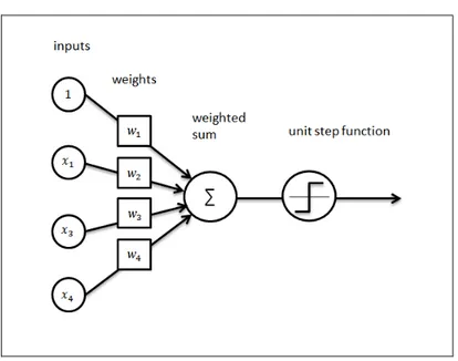
The history of neural networks is quite old. Rosenblatt (1958) was a psychologist and he proposed “the perceptron” which is a mathematical model heavily inspired by biological neurons in human brain. As we can see in Figure 2.1, the model has n binary inputs and exactly same number of weights. Each input value is multiplied by the corresponding
weight. If the sum of these products is larger than zero, the perceptron is activated and it outputs a signal whose value is generally +1. Otherwise it is not activated with an output value of 0. This is the mathematical model for a single neuron, the most fundamental unit for neural networks.
Figure 2.1: A diagram of the perceptron model
Since the perceptron model has a single output, it can perform just binary classification. A stronger structure called “a layer” has been formed with connecting many perceptrons in parallel fashion. Thus, this enables to work for classification tasks with many categories. This structure is called Single-Layer Perceptron or Single–Layer Neural Network.
However, single unit perceptrons are only capable of learning linearly separable tasks. Minsky and Papert (1969) famously showed that it is impossible for a single layer perceptron to learn a simple XOR function. They also stated that this issue could be overcame by adding intermediate layers called hidden layers. That architecture is now called Multi-Layer Perceptron or Multi-Layer Neural Network. But the real problem was that Rosenblatt’s learning algorithm did not work for multiple layers and nobody knew how to adjust the weights of hidden layers at that time. After a long stagnation period in artificial intelligence field, Werbos (1982) utilized the back-propagation
algorithm to train multi-layer neural networks. But its importance wasn't fully appreciated until the famous work of Rumelhart et al. (1986).
Cybenko (1989) proved in his universal approximation theorem that a neural network with 1 hidden layer can approximate any function, which means it can learn anything in theory. However, it is observed that deeper networks worked better in practice. In spite of the fact that nobody knows the real reason of this phenomenon, there are two main arguments. The first one is that multiple layers create the effect of hierarchical process. Therefore, deeper models should learn the desired function by combining several simpler functions. On the other hand, the second argument is that the number of units in a shallow network grows exponentially with task complexity. So in order to increase the capacity of a shallow network that much, the network might need to be very big, possibly much bigger than a deep network.
However, researchers did not have widespread success training neural networks with more than 2 layers. Because bigger networks require more computing resource, and that kind of large computational power is not commonly available at that time. Another obstacle is the lack of big and high-quality data. This causes the network to overfit on training data, resulting with failing to capture the true statistical properties. But the main problem with deep networks is so-called vanishing gradients; the more layers are added, the harder it becomes to update the weights because the error signal becomes weaker and weaker. Since the initial weights can be quite off due to random initialization, it can become almost impossible to learn the true features.
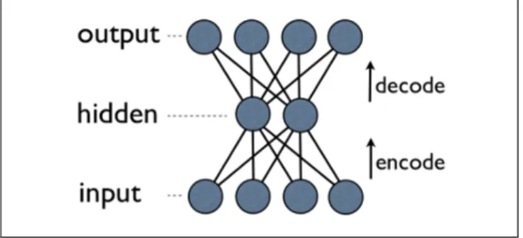
Deep learning era started in 2006. Deep learning is a just popularized name by community, emphasizing that researchers were now able to train many layer neural networks. There is no exact definition of the term “deep”, but it is often referred for having two or more hidden layers. Hinton et al. (2006) proposed a new weight initialization strategy called greedy layer-wise pre-training. Before training whole network with back-propagation, they individually trained each layer as autoencoders. Autoencoder is a neural network architecture which learns compressing the input and uncompressing that representation into something that closely matches the original data.
Figure 2.2: A view of autoencoder compression
Since autoencoders are generally shallow, they are less effected by vanishing gradient problem. They used this unsupervised technique to determine the network’s initial weights instead of random initialization. They showed that deep networks can be successfully trained with better weight initialization. Then in 2010, researchers realized that pre-training is not only way to train deeper networks; using different activations functions, regularization methods and architectures makes a huge difference for back-propagation.
2.3 CONVOLUTIONAL NEURAL NETWORKS
CNN is a type of feed-forward neural networks designed to work on spatial information such as images. It is heavily inspired from biological processes. According to their work on the visual cortex, Hubel and Wiesel (1959) proposed a featural hierarchy of cells. First, there are simple cells responding to low level features like edges and colors in their small receptive field, and then there are complex cells above them which are sensitive to higher level features such as shapes. As we go up in this hierarchy, cells are starting to sense more and more complex patterns.
CNNs use convolutional and pooling layers, different from standard feed-forward networks. In convolutional layers, a simple 2-dimensional convolution operation is performed for each filter. The number of filters in a layer is left to designer’s choice. The key thing is that the parameters of a filter are shared by all the possibly positioned neurons in the same layer. Therefore, learnt filters are independent from position information in the image. In general, a convolutional layer is followed by a pooling
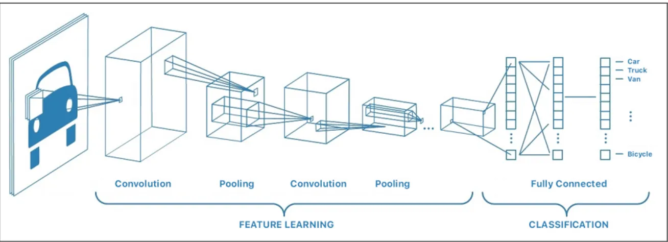
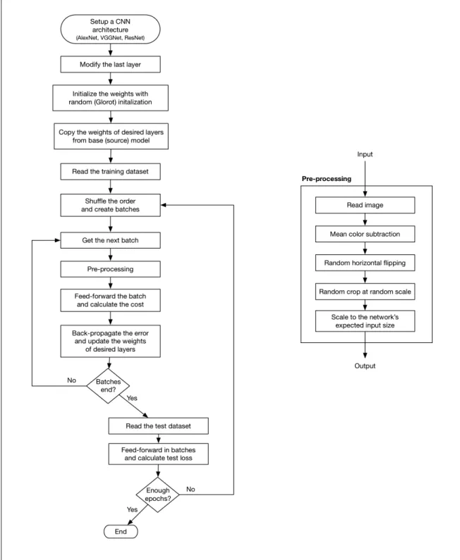
layer where 2-dimensional input is simply downscaled. The main purpose of this layer is reducing the number of parameters and controlling overfitting. These convolutional and pooling layers are get stacked on top each other to learn more and more complex features. The structure of a typical CNN can be seen in Figure 2.3. Subsequent to convolutional layers, there are fully-connected layers as we are familiar from feed-forward neural networks. In first fully-connected layer, highest-level image features are got flatten. Then, they are fed to next layers for desired task such as classification.
Figure 2.3: Structure of a typical convolutional neural network
Source: MathWorks
The first successfully applied CNN is LeNet (LeCun et al. 1998). It recognizes digits from 32x32 pixel images of hand-written numbers. Although this network achieved promising results, it did not get much attention at that time. Because this method could not be applied to more complex problems due to limited computer power and lack of large image datasets.
2.3.1 AlexNet
AlexNet is the first CNN that wins ILSVRC by outperforming the runner-up with about 10 percent margin (Krizhevsky et al. 2012). At that time, using handcrafted features was accepted as state-of-the-art methods in computer vision field. AlexNet has changed this with its groundbreaking success. From then on, all of the ILSVRC winners have been using CNNs.
Actually, its architecture is very similar to LeNet. It is a deeper and bigger network with 5 convolutional and 3 fully-connected layers. Needless to say, the dataset is much larger and consumer-level powerful graphic processing units (GPUs) had emerged. They proposed new techniques that have been still used today.
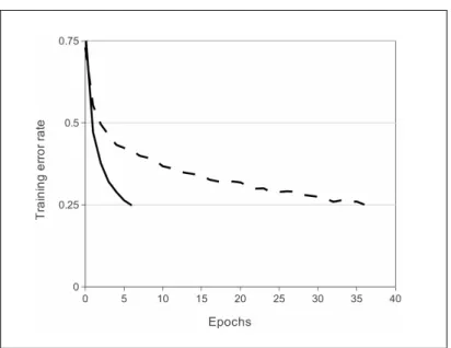
They used Rectified Linear Unit (ReLU) as non-linear activation function. It simply thresholds negative values to zero. They reported six times faster training time compared with conventional tanh activation function when training on CIFAR-10 dataset (Figure 2.4). ReLU is currently the most popular activation function just works best for most of the cases.
For regularization, they proposed dropout method. Krizhevsky et al. (2012, p.6) explain, “The neurons which are dropped out in this way do not contribute to the forward pass and do not participate in back-propagation.”. Its motivation is decreasing the dependence between neurons, so that they can learn more robust features. They reported that even though it increases the training time, the network was suffered from overfitting without dropout.
Figure 2.4: Training speed difference tanh (dashed) and ReLU activation functions
Another key point of this work is data augmentation. As mentioned earlier, ILSVRC contains 1.2M images which seems reasonably large. However, AlexNet uses offline patch extraction and horizontal reflection techniques to artificially increase the size of dataset by a factor of 2048. They stated that such big networks overfit easily without data augmentation.
2.3.2 VGGNet
VGGNet is another famous CNN featuring pretty homogenous and deeper architecture (Simonyan-Zisserman 2014). AlexNet and ZFNet, which is the winner of ILSVRC 2013, used large convolutional filters such as 11x11 and 7x7 in the first convolutional layers, while VGGNet uses just 3x3 filters across all the convolutional layers. It should be noted that 3x3 is the smallest filter size to capture the notion of left/right and up/down. They show that larger receptive fields can be simulated by stacking 3x3 filters on top of each other. A stack of two 3x3 convolutional layers has an effective receptive field of 5x5. This also decreases the number of parameters from 25 to 18. Similarly, a combination of three 3x3 filters have 27 parameters and it simulates a 7x7 filter which would have 49 parameters.
Beside of having less parameters, stacking these 3x3 filters acts like a regularization by forcing larger filters to be formed through multiple 3x3 filters. They also reported faster training times comparing with AlexNet due to this implicit regularization. Additionally, these stacks use more ReLU layers instead of just one, which provides more discriminative decision function.
VGGNet architecture proposes 6 different network configurations. When the architecture is examined from higher perspective, it is very similar to AlexNet. It has 5 convolutional blocks following by 3 fully-connected layers. Each configuration just differs at the number of stacked 3x3 layers in these convolutional blocks. These configurations have 11, 13, 16 and 19 actual layers and each network is denoted as “VGG-⟨number of layers⟩” such as VGG-16.
VGGNet uses an online data augmentation pipeline featuring random cropping at random scale between a fixed interval. The main idea is simple, a scale interval is firstly defined such as (S1, S2). A random integer S is picked up between S1 and S2. Then, both width and height of the input image is scaled to S. Finally, the image is cropped at a random position in size of 224x224 pixels which is the input size of VGGNet. They achieved up to 3 percent better scores with this technique when compared with fixed-size cropping. They also used random horizontal flipping just like AlexNet.
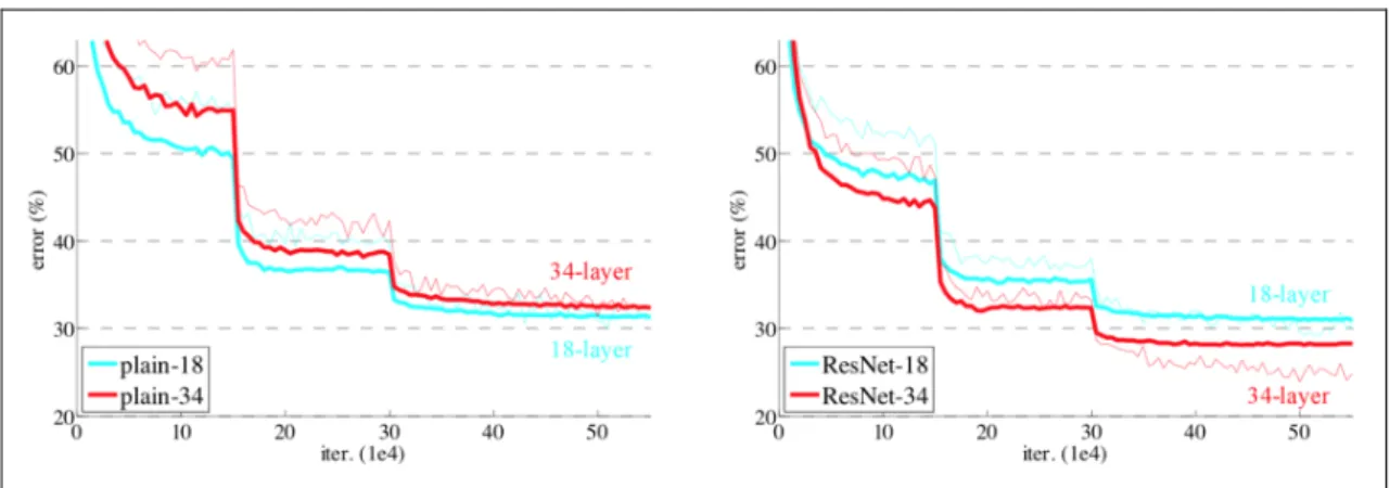
2.3.3 ResNet
Another fascinating CNN architecture is ResNet proposed by He et al. (2015). They heavily investigate the effect of the network depth. They observed that deeper plain networks have higher training error, and thus test error. This phenomenon can be seen in Figure 2.5. To overcome this problem, they proposed residual blocks which has skipped connections between every following two convolutional layers. The main idea of this shortcut connections is to prevent performance degradation by preserving more information about input as the network getting deeper. Another benefit of residual blocks is decreasing the effect of infamous vanishing gradients problem.
Figure 2.5: Training of plain networks (left) and residual networks (right) on ImageNet
Source: He et al. 2015, Figure 4
They use 18, 34, 50, 101 and 152 layered networks using same residual network architecture. They achieved 3.57 percent top-5 error with the deepest 152-layer
configuration by surpassing human-level accuracy. Human error rate is estimated 5.1 percent (Russakovsky et al. 2015).
They even experimented with 1202-layer network, however they observed worse performance compared to 101-layer network even though their training accuracies are similar. They argued that overfitting could be the reason of this. Nevertheless, there are still open problems for such aggressively deep networks.
2.4 DISTANCE METRIC LEARNING
Distance metric learning or similarity learning is a supervised machine learning technique closely related to regression. The task is learning a distance function over labeled inputs, so that all the same classes positioned close to each other while different classes are far apart in the output representation space. This process is also known as “embedding”.
After getting these embeddings, many computer vision tasks become straightforward. Verification becomes just a distance check, classification and recognition task becomes simple k-NN problem. Additionally, standard clustering algorithms such as k-means can be applied in the embedding space for unsupervised learning.
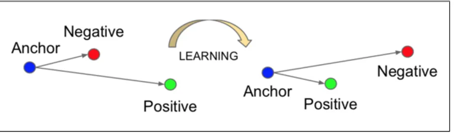
This technique adopted to neural networks by Siamese network architecture (Bromley et al. 1993). They used two identical sub-networks to process two different inputs and a unified output layer compares their outputs for signature verification task. The sub-networks share the weights, so it is trained to produce similar outputs for similar inputs. However, this approach compares just two samples at a time. Hoffer et al. (2015) proposed triplet loss as an improvement to Siamese networks architecture. The network takes a triplet of an anchor, a positive and a negative input at a time. It tries to minimize the anchor’s distance to positive sample, while maximizing the distance to negative sample (Figure 2.6).
Although triplet approach seems intuitive, it comes with own difficulties. According to their FaceNet work of Schroff et al. (2015), triplet selection is extremely important to achieve good results.
Figure 2.6: Triplet loss minimizes the distance to positive sample while maximizing the distance to negative
Source: Schroff et al. 2015, Figure 3
FaceNet architecture proposes two online triplet mining strategies. First one is “hard selection” where the hardest positive and the hardest negative sample in the batch are selected for each sample. The other selection method is “semi-hard negative selection”, because they observed that too hard negatives can lead to bad local minima in early stages of training. However, batch generation is still open problem because positive and negative samples are selected from current batch. FaceNet uses very large batches with thousands of samples as a workaround for this issue, which makes impossible to train on GPUs. This issue is addressed by Hermans-Beyer et al. (2017), they use PK-style batch generation where random P identities are sampled, then selected random K images without replacement. They also showed that the hardest triplet selection method performs better with this batch generation strategy.
2.5 TRANSFER LEARNING & FINE-TUNING
Transfer learning is quite an old idea in machine learning field. As the main purpose of pattern recognition is to learn how to generalize input data, transfer learning is investigating how to use this generalized feature knowledge on a different task or problem.
As mentioned earlier, CNNs are designed to work like animal visual cortex system. There is a hierarchy of simples cells to more complex ones that are responding more and more complex patterns. The convolution filters at the first layer of AlexNet, which is trained on ImageNet, can be seen in Figure 2.7. It turns out that these filters are very similar to the ones that are being hand-engineered by computer vision community for over 30 years.
This is the motivation behind transfer learning idea, there is no need to learn same low-level features again and again. Transferring these features works great on small datasets, because small datasets are insufficient for such big networks to learn this generic features. Moreover, networks converge much faster from when they trained from scratch. If training times are considered, many modern networks require 2-3 weeks to train on ImageNet with multiple GPUs (Simonyan-Zisserman 2014, Krizhevsky 2012). So, this technique also makes rapid experimenting possible.
Figure 2.7: AlexNet’s first-layer convolution filters learnt from ImageNet
Source: Krizhevsky et al. 2012, Figure 3
Although its many benefits, Hermans-Beyer et al. (2017) stated, “Using pre-trained models does not allow for the exploration of new deep learning advances or different architectures.”.
There lots of way to transfer learning between CNNs. The usual approach is to copy first n layers of source model to first n layers of target model, and then train the rest of network. However, the number how many layers to be transferred is open question. Likewise, initial weights of the layers to be trained can be transferred from pre-trained model instead of starting randomly which is called “fine-tuning”. These choices are left to implementer.
Yosinski et al. (2014) performed comprehensive experiments on these transfer learning methods. They divide ImageNet dataset into two groups that each has approximately 500 non-overlapping classes. They utilize two separate AlexNet and train on split datasets from scratch, they called these models “baseA” and “baseB” respectively. For both models, every possible first n-layer is transferred to both blank A and B networks and then they train the rest of network from scratch. They also repeat this experiments with fine-tuning method. According to their work, fine-tuning recovers most of the lost (not transferred) features when transferring to “selfer” networks (baseA to A, or baseB to B). The most interesting part of the study is when they apply transfer learning between cross networks (baseA to B, or baseB to A), they observed better performance compared with their base models. This phenomenon occurs because networks generalizes better with a base. We also experiment on these methods in the next chapter.
2.6 MARVEL DATASET
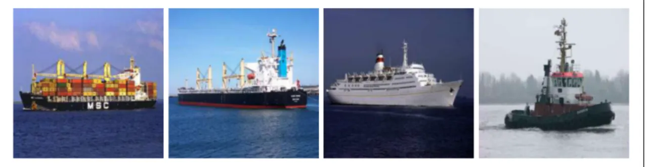
MARVEL is a public dataset containing 2M ship images, it is created to fill the absence of a benchmark dataset specifically designed for marine vessel classification, verification and recognition tasks by Gundogdu-Solmaz et al. (2016). Ship images and their annotations including vessel type and IMO number, which is a unique identification number of a ship, are taken also from ShipSpotting website. There are 109 different vessel types in total, however the dataset is not balanced. So they utilize a semi-supervised clustering scheme to combine similar vessel types. They ended up with 26 more balanced superclasses. Some examples can be seen in Figure 2.8.
Figure 2.8: Some samples of MARVEL dataset. Superclasses from left to right; container ship, bulk carrier, passenger ship, tug
For superclass classification task, 140K unique images in 26 superclasses are gathered after semi-supervised clustering scheme. For each superclass, they selected 8192 and 1024 images for training and test set respectively. For the superclasses that have insufficient samples, they generate more images by cropping different patches of images. Finally, the training and test set contain about 212K and 26K examples respectively. This dataset is referred as superclass dataset.
Prior to verification and recognition tasks, 8000 vessels with unique IMO number are selected such that each vessel has 50 sample images. They divide these vessels into 2 groups by preserving vessel type distribution, 4035 vessels for training and 3965 for test set. We refer these datasets IMO training set and IMO test set respectively. There are still 109 vessel types in among these 400K images.
For verification task, 50K positive and 50K negative pairs selected randomly from IMO training set, resulting in 100K total pairs. It is called as verification train set. Verification test set is collected in the same way, but from IMO test set.
Lastly for recognition task, they decided to perform recognition among individual vessel types due to computational complexity, because there are 3965 ships in IMO test set. Therefore, 29 vessel types are extracted so that each type has at least 10 unique ships and each ship contains 50 sample images. They split each vessel type into 5-fold cross-validation scheme such that each vessel has 40 training and 10 test images.
3. MARITIME VESSEL CLASSIFICATION
In this chapter; AlexNet, VGGNet and ResNet architectures are trained for vessel superclass classification task while experimenting on transfer learning techniques. The task is straightforward; for a given ship image, the goal is to identify its vessel type among 26 superclasses. There are also other experiments for investigating the effects of dropout and data augmentation. In the next section, the used dataset is described in detail. Then, the main experimental methods utilized are given with the motivations behind them, followed by obtained results. Lastly, our scores are compared with best results on MARVEL superclass dataset.
3.1 DATASET
Gundogdu-Solmaz et al. (2016) provided a Python script to download MARVEL dataset. However, some images are deleted from the website and some of them could not be downloaded due to operational reasons. For superclass classification, 137293 unique images are downloaded and our train set contains 211876 images while test set contains 26491 images. In original MARVEL superclass dataset, 212992 and 26624 images are reported for training and test set respectively in total of 140K unique samples. So we have about a thousand less samples, which can be ignored. The resolution of all downloaded images is 256x256 pixels.
3.2 METHOD
Gundogdu-Solmaz et al. (2016) trained an AlexNet from scratch on this dataset. To emphasize that score, they also used a pre-trained VGGNet to extract features from the penultimate layer and dimensionality of extracted features is reduced to 256 with principal component analysis (PCA) method. Then they train a multi-class support vector machine (SVM) with the half of training set due to computational complexity.
Instead of training from scratch, we use different transfer learning techniques. In addition to AlexNet, VGG-16 and ResNet-50 networks are utilized which all are pre-trained on ImageNet.
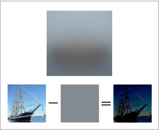
3.2.1 Preprocessing
Mean color subtraction and random horizontal flipping are used as the basic preprocessing methods. First, the mean image of superclass train set is calculated. As we can see from Figure 3.2, there is a dark colored blob in the center where ships are generally positioned in images. After acquiring the mean image, its mean color is calculated as (132.27, 139.65, 146.97) in BGR color space which is a grayish color. This mean color is subtracted from the input image (Figure 3.2). Then it is horizontal flipped with 50 percent randomness. Before feeding them into network, they are scaled to expected input size of the networks which is 227x227 for AlexNet, 224x224 for VGGNet and ResNet.
Figure 3.2: Mean image of superclass train set (above), mean color subtraction (below)
Additionally, we experiment with random cropping at a random scale, which is described in Section 2.3.2, with three different scaling intervals; (228, 256), (228, 286) and (256, 286).
3.2.2 Training
Pre-trained AlexNet, VGG-16 and ResNet-50 models are taken, and their 1000-neuron output layer is replaced by 26-neuron layer. Because we want to classify 26 vessel superclasses.
The layers to be trained from scratch are initialized with Glorot initialization (Glorot-Bengio 2010). On the other hand, the layers to be fine-tuned are initialized with transferred weights from a source model.
At first, stochastic gradient descent (SGD) is used as optimizer with 0.01 learning rate. Shortly after, we have switched to ADAM optimizer due to its much faster convergence. For all the results reported in this project, ADAM optimizer is used. We use 0.001 learning rate by default, but it is decreased in some cases for more stabilized training which will be stated explicitly.
According to our initial observations, training loss generally converges before 10th epoch and does not improve afterwards. But most of experiments, network is trained for 20 epochs anyway.
If the network contains dropout layers, 0.5 is used if not specified explicitly. To investigate the effect of dropout, we also experiment with four different dropout values; 0.2, 0.35, 0.65 and 0.8.
3.2.3 Transfer Learning & Fine-tuning
First, we apply plain transfer learning to a AlexNet network by copying the first n layers from a model pre-trained on ImageNet and training the last (8 - n) layers from scratch. For instance; if we are training last two layers of network, first 6 layers are copied from pre-trained model and they are fixed (or frozen) during training. This training scheme is denoted as fc7+. The number 7 stands for 7th layer (which is a fully-connected layer), and plus sign at the end implies that 7th and following layers are being trained. Similarly, if we transfer the first two layers from pre-trained model and train the rest, it
is denoted as conv3+ (3rd layer is a convolutional layer). Please notice that, the layers to be trained are initialized with Glorot initialization. Also the last layer could not be copied from pre-trained model, because we have modified it in order to classify 26 vessel superclasses.
Figure 3.3: Difference of plain transfer learning (above) and fine-tuning (below) techniques, exemplified for conv3+ training scheme on AlexNet.
In the next experiment; we repeat the same experiment described above, but with fine-tuning approach this time. So, the layers to be trained are initialized with the transferred weights from pre-trained model. It should be noted that all the layers except the final layer are transferred for every training scheme (Figure 3.3).
3.2.4 Orientation-Specialized Networks
Ensemble of specialized networks approach is also investigated. For this experiment, we have decided to use ship orientation information. We assumed that these orientation-specialized networks could improve classification performance. Therefore, we define four orientations by using position of the camera relative to subject ship. These orientations can be seen in Figure 3.4. Since there are no orientation labels for superclass dataset, and manually labelling 137K images would be infeasible, we employ a ResNet network to do most of the heavy-lifting. 1250 samples for each orientation are manually labelled, resulting in a total of 5000 images. We randomly split this orientation dataset such that each orientation has 1000 training and 250 test images. We fine-tuned a ResNet-50 network pre-trained on ImageNet, and got 96.7 percent test accuracy. Then, we ran this network on whole superclass dataset to acquire their orientation labels. These orientation labels were manually corrected with human supervision.
Figure 3.4: Orientation convention according to camera position relative to subject ship
In the end, superclass dataset is divided into four orientation-specific subsets which we refer as orientation dataset from 1 to 4 respectively. After these preparation steps, we fine-tune AlexNet, VGG-16 and ResNet-50 networks (pre-trained on ImageNet) for each orientation. It should be noted that random horizontal flipping is not used, because it changes the orientation. Additionally, we merge horizontally symmetrical orientations into two groups and repeat same experiments. Thus, random horizontal flipping can be used in that way.
3.3 EXPERIMENTAL RESULTS
All the experiments are conducted on a high-end desktop computer. It has Intel i5-6600K CPU, 16GB memory, NVIDIA GTX 1080Ti with 11GB memory. Operating system is Ubuntu 16.04 LTS. TensorFlow 1.1 and SciKit-learn 0.18.2 libraries is used on Python 2.7 programming environment. The results and findings of each conducted experiment are covered in the following sections.
3.3.1 Transfer Learning & Fine-tuning
The results of training accuracies can be seen in Table 3.1. When just the last layer (fc8) is trained, we observed that the network’s performance on training set stuck at 63 percent. This is normal because it shows that there is no capacity to learn the training set completely. As more layers being trained, training accuracy increases rapidly as expected. When we train with conv5+ scheme, networks reach enough capacity to classify almost all of the training set correctly with 99 percent accuracy. It can be also seen that instead of plain transfer learning, fine-tuning improves the training with a subtle difference.
Table 3.1: Training accuracies of different transfer learning techniques (%)
Training Scheme Plain Transfer Learning Fine-tuning
fc8 63.21 - fc7+ 95.13 96.44 fc6+ 96.62 98.80 conv5+ 99.56 99.66 conv4+ 99.78 99.81 conv3+ 99.84 99.85 conv2+ 99.87 99.90 conv1+ 99.90 99.91
If we look at resulting test accuracies in Table 3.2, they are more interesting. When we train just the output layer with plain transfer learning, the network achieved 52.97 percent test accuracy. As we train more layers, test accuracy increases as expected, but up to conv3+ scheme. It should be noticed that training more layers from scratch means transferring less layers from pre-trained model. With conv2+ scheme, the network’s score dropped 0.8 percent. If we go further with conv1+ scheme, which is equivalent to training the whole network from scratch, the score drops 3.09 percent more.
However, we saw that applying fine-tuning technique instead of plain transfer learning fixes this performance degradation. The best score is obtained when fine-tuning with
conv3+ scheme just like plain transfer learning. There is no significant performance
change observed when trained with conv2+ and conv1+ schemes. After this point, test scores almost stabilized unlike plain transfer learning. This phenomenon can be seen clearly in Figure 3.5. Another important result is that fine-tuning all the layers scored 6.41 percent better than training the network from scratch.
Table 3.2: Test accuracies of different transfer learning techniques (%)
Training Scheme Plain Transfer Learning Fine-tuning Difference
fc8 52.97 - - fc7+ 61.59 61.55 -0.05 fc6+ 64.37 65.57 1.20 conv5+ 65.07 66.98 1.91 conv4+ 66.27 68.10 1.83 conv3+ 67.16 69.72 2.56 conv2+ 66.36 69.39 3.03 conv1+ 63.27 69.68 6.41
Figure 3.5: Comparison between plain transfer learning and fine-tuning over training depth
3.3.2 Dropout
As we can see from the results presented in Table 3.3, best scores are obtained with average dropout values such as 0.35, 0.50 and 0.65. When it is aggressively increased or decreased, performance drops more than 1 percent.
Table 3.3: Test accuracies for different dropout values
Dropout Probability Best Score
0.20 68.52
0.35 69.66
0.50 69.72
0.65 69.75
0.80 68.55
3.3.3 Random Crop at Random Scale
The results can be seen in Table 3.4. Random scaling significantly improved the performance. However, as input image is being more up-scaled, test scores started to decrease. This is expected because the network sees quite small part of the images, so that it cannot make generalization. We observed that fairly small up-scaling such as
(228, 256) works the best, if AlexNet’s 227x227 input size is considered.
Table 3.4: Test accuracies for different random cropping scale intervals
Scale Interval Best Score
No random crop 69.72
(228, 256) 71.17
(228, 286) 70.77
3.3.4 VGGNet and ResNet
In this experiment; VGG-16 and ResNet-50 will be fine-tuned layer by layer with the best experiment techniques including random cropping, and their performance will be compared with AlexNet. When training conv2+ and afterwards for VGG-16, also
block1+ for ResNet-50, batch size is decreased from 128 to 64 because of high memory
requirements.
Table 3.5: Test accuracies for VGG-16 (%)
Training Scheme Best Score
fc8 51.85 fc7+ 59.87 fc6+ 66.01 conv5+ 73.13 conv4+ 75.65 conv3+ 76.10 conv2+ 76.21 conv1+ 76.60
Table 3.6: Test accuracies for ResNet-50 (%)
Training Scheme Best Score
fc6 58.92 block5+ 73.16 block4+ 75.24 block3+ 75.37 block2+ 75.24 block1+ 76.04
As we can see from the results in Table 3.5 and Table 3.6, the best results were obtained when fine-tuning all layers for both networks. These networks achieved about 5 percent improvement over AlexNet, whose best score is 71.17 percent. Also it should be noted that after conv4+ for VGG-16 and block4+ for ResNet-50, the performance improved at
3.3.5 Orientation-Specialized Networks
In this experiment we have observed the networks that fine-tuned on merged datasets performed better than single orientation specialized networks (Table 3.7). In fact, the whole superclass dataset worked the best for all network architectures. In this manner, we can clearly say that this orientation-specialized network approach did not work.
Table 3.7: Test accuracies of orientation-specialized networks (%) Orientation Dataset AlexNet VGG-16 ResNet-50
1 68.64 72.02 72.04 2 69.63 74.39 72.19 3 68.63 74.18 72.74 4 68.29 72.26 71.98 1+4 69.05 74.80 72.31 2+3 65.16 76.23 74.18 1+2+3+4 71.13 76.52 75.99
We argue that this is because orientation information is already learnt and generalized by networks. By splitting the dataset according to orientations, we are not helping. Instead, we are just decreasing the dataset size which causes performance degradation.
3.3.6 Transferring Learning from Relevant Source
As a final experiment for vessel classification task, we have fine-tuned some VGG-16 networks pre-trained on other MARVEL datasets which will be described in next chapter, Section 4.3. Although this seems like against to main purpose of benchmarking, it will help us to make a comparison between generic and relevant learning transfer sources.
We have two pre-trained models, both of them is trained on IMO train set. But first one is trained for 109 vessel types, while the other one is trained for 3980 vessel identities (Section 4.3). The results can be seen in Table 3.8. We have observed that choosing a
relevant source model improved the performance for this dataset with more than 2 percent when compared to ImageNet.
Table 3.8: Test accuracies of different pre-trained models used for fine-tuning (%)
Source Model Best Score
ImageNet 76.60
BASE-109 (109 vessel types) 78.79
BASE-3980 (3980 vessel identities) 78.56
3.4 COMPARISION WITH THE STATE-OF-THE-ART
A comparison between our scores and theirs (Gundogdu-Solmaz et al., 2016) can be seen in Table 3.9. They got 73.14 percent accuracy by training an AlexNet from scratch. However, we achieved 71.10 percent even with fine-tuning approach. We saw that VGG-16 performed the best with 76.60 percent accuracy, followed by ResNet-50 with 76.04 percent.
Table 3.9: Superclass classification scores compared with state-of-the-art (%)
Model Best Score
VGGNet features + SVM [1] 53.89
AlexNet [1] 73.14
AlexNet (ImageNet + fine-tuning) 71.19
VGG-16 (ImageNet + fine-tuning) 76.60
ResNet-50 (ImageNet + fine-tuning) 76.04
VGG-16 (BASE-109 + fine-tuning) 78.79
4. MARITIME VESSEL VERIFICATION
In this chapter, we focus on vessel verification task which is simply deciding whether two images belong to same ship or not. Experimental setup is almost identical with classification experiment, except for the dataset. First, we prepare some base models to be fine-tuned later on distance metric learning experiments which is described in following section.
4.1 DATASET
As mentioned earlier in Section 2.6, we will use MARVEL IMO dataset. Verification dataset will also be used, which is already utilized from IMO dataset. The properties of the datasets can be seen in following Table 4.1 and Table 4.2. Just like superclass dataset, we have negligible missing data.
Table 4.1: Properties of MARVEL IMO dataset
Reference Downloaded
Vessel type in both sets 109 109
# of unique vessels in training set 4035 4001
# of unique vessels in test set 3965 3943
# of images in training set 201750 197832
# of images in test set 198250 194429
Table 4.2: Properties of MARVEL verification dataset
Reference Downloaded
# of positive pairs in training set 50000 48647
# of negative pairs in training set 50000 47941
# of positive pairs in test set 50000 48689
4.2 METHOD
Gundogdu-Solmaz et al. (2016) trained an AlexNet on IMO training for 109 vessel type labels from scratch. They used this network as feature extractor by probing activations in the penultimate layer, which is a 4096-dimenson vector. After acquiring the features of verification dataset, they reduced the dimensionality to 100 with PCA. All the pairs in verification training set are concatenated into 200-dimensional vector, and they used SVM and nearest neighbor (NN) classifier.
Instead, we apply a distance metric learning approach to this task. Just VGG-16 architecture is utilized due to its success in classification task. We fine-tune it by using triplet loss as explained in Section 2.4. It should be noted that triplet loss enables end to end training. In theory; if the distance between a pair in embedding space is smaller than a threshold, they belong to same vessel, and vice-versa. This removes the need of additional classifier. However, we also make experiments with SVM.
We have tried directly fine-tuning a VGG-16 pre-trained on ImageNet with triplet loss, but the results were very poor. Parkhi et al. (2015) stated these kind of difficulties for triplet loss. In their work, they trained a CNN as a classifier first. Then they replaced the last layer with desired embedding layer and they fine-tuned just this layer with triplet loss. They reported that this technique makes training significantly easier and faster. Therefore, some base models are prepared to be fine-tuned with triplet loss which are explained in the next section.
To fine-tuning with triplet loss, we generally followed common configurations. We used 128-dimensional embedding space. Output of the network is normalized by using L2 normalization. Since the maximum distance in L2 normalized space is 2, we choose the margin of triplet loss as 1. It is simply the desired distance between positive and negative samples.
As discussed earlier in Section 2.4, triplet selection is critically important. In trial and error phase, we have observed the approach of Hermans-Beyer et al. (2017) works the best. Therefore, we used batch hard triplet selection strategy and also PK-style batch
generation method. We also followed a common practice by taking K = 4. If we consider our default batch size of 128, there will be P = 32 unique vessels containing K
= 4 images each.
However, choosing P identity from dataset is still open question. For face verification, the most common way is picking random. But we can use vessel type information to choose vessels in same category together. So, there would be much harder triplets in a batch when compared to random selection. However, this approach did not work in practice. Hermans-Beyer et al. (2017) explained the reason of this issue is because network selects outliers so often that it is unable to learn normal associations. Therefore, we ignored vessel type information and selected vessels randomly.
For evaluation, Euclidian pair distances in embedding space are calculated for verification test set. Then, simple linear regression is run to determine best threshold value that separates positive and negative pairs. It should be noted that verification training set is not used in this configuration.
4.3 BASE MODEL PREPARATION
We have decided to train a network that classifies 4001 unique vessels in IMO training set. Since the training and test sets of IMO dataset contain different vessels, we need a test dataset for evaluation purposes. First, we took out the vessels which contains less then 10 images. Then, 5 images are extracted randomly for each vessel. As a result, we had 177856 training and 19935 test images for total of 3980 unique vessels.
After preparing this dataset, we utilized a pre-trained VGG-16 on ImageNet, and we have attempted to fine-tune it. Even though we have tried lots of different configurations, the network did not converge.
We went back to IMO training set, and we have fine-tuned another pre-trained VGG-16 for 109 vessel types. The network performed fairly well with 78.67 test accuracy. This score is even higher than what we achieved for classification task with just 26
superclasses. However, it should be noted that this dataset is not balanced. Nevertheless, this model is referred as BASE-109.
Then, we have tried again to fine-tune a VGG-16 network for 3980 vessels, but this time we used BASE-109 model instead of ImageNet. This model managed to achieve a promising result with 61.85 percent test accuracy. Likewise, we refer this model as BASE-3980.
4.4 EXPERIMENTAL RESULTS
After preparing base models, we experiment on training depth and embedding size of triplet loss. We will also compare the performance of end-to-end training enabled by triplet loss and an additional SVM classifier. The results and findings of each conducted experiment are covered in the following sections.
4.4.1 Training Depth
For superclass classification task, we have seen that fine-tuning prevents performance degradation as more layers being trained. So, whole network can be trained to obtain best results if computing power requirements can be afforded. However, we have observed that networks oscillated immediately and they did not converge even after 5 training epochs.
We used incremental fine-tuning to overcome this issue. First, we trained just the last layer with triplet loss. After seeing convergence and stabilization, we stopped the training and started fine-tuning more layers.
Table 4.3: Verification test results of different training depths (%)
Training Scheme Accuracy Precision Recall F1 Score
fc8 92.89 92.92 92.92 92.92
fc6+ 92.08 92.12 92.12 92.12