Rate-distortion based piecewise planar 3D scene geometry representation

RATE-DISTORTION BASED PIECEWISE PLANAR 3D SCENE GEOMETRY

REPRESENTATION

Evren ømre, A. Aydın Alatan and U÷ur Güdükbay

Department of Electrical & Electronics Engineering, METU

Balgat 06531 Ankara, TURKEY

Department of Computer Engineering, Bilkent University

Bilkent 06533 Ankara, TURKEY

E-Mail: {e105682@, alatan@eee.}metu.edu.tr, gudukbay@cs.bilkent.edu.tr

This work is funded by EC IST 6th Framework 3DTV NoE (Grant No: FP6-511568) and partially funded by TÜBøTAK under Career Project 104E022

ABSTRACT

This paper proposes a novel 3D piecewise planar reconstruction algorithm, to build a 3D scene representation that minimizes the intensity error between a particular frame and its prediction. 3D scene geometry is exploited to remove the visual redundancy between frame pairs for any predictive coding scheme. This approach associates the rate increase with the quality of representation, and is shown to be rate-distortion efficient by the experiments.

Index Terms— Rate-distortion optimal 3D

representation, piecewise planar 3D reconstruction.

1. INTRODUCTION

Dense 3D scene representations are essential in 3DTV applications, due to their potential to eliminate the visual redundancy between the sequences of a multi-view video and to improve the compression rate of a 3DTV bit-stream. Obviously, the realization of this goal requires an efficient and accurate representation of the 3D structure. Hence, this problem can be studied within the rate-distortion framework.

Among the earliest attempts to fulfill the above requirement is [1], in which 3D scene structure is extracted in a rate-distortion optimal sense, by jointly optimizing the number of bits to encode the dense depth field and the quality of the reconstructed frame, via a Markov random field formulation. This method, while successful, still leaves room for further improvement in 3D scene representation.

2. DENSE 3D SCENE REPRESENTATION

A dense 3D reconstruction can be described either by a point-based representation, as a depth-map defined on the same lattice with the reference frame, or as a mesh-based

piecewise planar surface, or by a volumetric representation, such as voxels [9]. However, planes offer distinct advantages, as basic representation elements. Man-made environments and even many natural scenes could be well-approximated by polygonal patches. Besides, planes can be succinctly parameterized. Finally, they are algebraically easy to handle, providing significant computational savings.

The considerable body of research on piecewise planar scene representations can be analyzed in two major classes. In the first approach, a planar surface is fit onto an irregular 3D point cloud. A good example is presented in [3], in which the point cloud is divided into cells and a dominant plane is identified in each cell via RANSAC. An equivalent procedure is described in [2] to determine the homographies induced by scene planes from 2D correspondences.

The use of triangular meshes, specifically Delaunay triangulation, due to its certain optimality properties [4], characterizes the second approach. There exist successful algorithms that can construct a triangular mesh from an irregular 3D point cloud [5]. However, image-based triangulation (IBT) techniques [6] are one step beyond, as they are also capable of incorporating the intensity information. The basic algorithm utilizes edge swaps on a triangular mesh, to minimize the intensity prediction error of an image of the scene, acquired by a known camera [6]. In [7], a simulated annealing procedure, equipped with a rich arsenal of tools in addition to edge swap, is employed. In the algorithm proposed in [8], a similar idea is used to represent a disparity map. However, it differs from the others by adding vertices to locations where the prediction error is largest, instead of simplifying a complex mesh.

Since IBT methods construct the mesh using the 2D projection of the 3D point cloud, they are prone to erroneous connections. However, the vertices of the mesh alone are sufficient to represent a Delaunay triangulation, unlike irregular-shaped planes generated by the plane-fitting

V - 113

process. Moreover, rendering of triangular meshes are readily supported by hardware. These advantages justify the choice of triangular meshes in this study.

In this paper, a coarse-to-fine, 3D piecewise planar reconstruction algorithm is proposed. The algorithm requires two images of the scene and the corresponding cameras as input, initially obtains a coarse mesh, and is guided by the prediction error to determine which parts of this mesh structure require a refinement.

3. PIECEWISE PLANAR 3D RECONSTRUCTION IN RATE-DISTORTION SENSE

3.1. Motivation

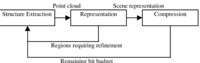
In order to find a rate-distortion efficient representation, a sequential minimization algorithm can operate either in a fine-to-coarse or coarse-to-fine fashion. The former leads to a more complex error surface along with the computationally inefficient practice of extracting information only to discard later on. Therefore, a coarse-to-fine approach is adopted as it not only avoids both of the above issues, but is also suitable for progressive coding and the construction of scalable bit streams. The rules that identify such an algorithm are those governing the location and the amount of refinement. The location is chosen to achieve maximal reduction in the distortion for the representation, while, in a compression scenario, the available number of bits, or rate, limit the amount of refinement. Figure 1 illustrates these ideas.

In this study, rate is defined as the number of vertices in the mesh. As for distortion metric, the choice is not straightforward. PSNR is the most popular distortion metric in the literature, although, it is oversensitive to geometric errors. Moreover, minimization of such an image-based error, when coupled with erroneous camera estimates, causes a projective distortion in the structure estimate. The alternative is geometry-based error metrics, measuring the discrepancy between the point cloud and the scene representation.

The minima of both of the above metrics should coincide when accurate camera matrices are available. In their absence, minimizing the image distortion transfers the error to the structure and vice versa. This observation explains the popularity of PSNR in novel view synthesis and image prediction problems [1].

3.2. Proposed Method

The proposed algorithm aims to build a rate-distortion efficient and accurate 3D scene geometry representation. The distortion is measured as the prediction error of the intensity values of a target image from a reference image. The minimal input to the algorithm is two frames, from which the projective camera matrices, and an initial 4-8 vertex mesh bounding the target image (required by the incremental Delaunay triangulation algorithm), can be estimated. However, the algorithm is capable of making use of any available projective camera matrices and mesh.

A cycle in the algorithm starts by finding a patch that requires refinement. To this aim, a prediction of the target image is computed by transferring the pixels in the reference frame to the image plane of the camera corresponding to the target frame, via the homographies induced by the planar patches in the current representation. The patch, whose corresponding region in the target image has the largest error, is chosen for refinement.

The local scene representation is refined by adding a vertex to the chosen patch. In order to determine the vertex position, the patch is projected to the target and the reference frames to define the region-of-interests (ROIs). In each ROI, a set of salient features are extracted by Harris corner detector. These features are matched by guided matching; a technique that uses the fact that the fundamental matrix, computed from the camera matrices, constrains the possible matches of a feature in an image to lie on a line in the other [11]. For each matching pair, there is a corresponding 3D vertex. Among these vertices, the one that has the largest discrepancy with the current scene geometry estimate is added to the representation. The discrepancy is measured by symmetric transfer error [11], a projective metric, as it dispels the need to use calibrated cameras. The metric is defined as

(

)

(

)

where x1 and x2 are the homogeneous coordinates of the

matching pair and H is the homography induced by the planar patch, relating the ROIs.

The new vertex is added to the representation, only if it improves the representation quality; otherwise, it is rejected. The procedure is repeated until either the intensity prediction error converges, or the available bit budget is completely used up.

The sequential stage of the algorithm, described above, is followed by the non-linear refinement stage. The representation is parameterized by the cameras and vertices, and the prediction error is minimized using gradient-descent.

The flow of the algorithm is presented below.

Structure Extraction Representation Compression Point cloud Scene representation

Regions requiring refinement Remaining bit budget

Figure 1: 3D reconstruction in rate-distortion framework.

Algorithm: Piecewise-Planar Reconstruction

Input: Reference and target images, initial mesh (optional),

and the associated cameras (optional)

1. Until the prediction error converges or the bit budget is

depleted

2. Transfer the 2D points in the reference frame to the

target frame, and compute the intensity prediction error in the regions corresponding to each planar patch.

3. Project the patch with the largest prediction error to the

images to determine the ROIs. Extract new features and construct a correspondence set via guided matching.

4. Compute symmetric transfer error for each feature pair

in the set. Determine the pair with the largest transfer error, and add the corresponding 3D vertex to the mesh.

5. Go to Step 1.

6. Further refine the representation by non-linear

optimization.

4. EXPERIMENTAL RESULTS

The algorithm is first tested on “Cube”, a synthetic scene with 9 surfaces and 12 vertices, and for which the ground-truth for both the cameras and the geometry is available. In order to assess the effect of noise, the ground-truth values are perturbed randomly with a certain percentage of their original values. The reference, target and predicted images are presented in Figure 2, along with the error images at different stages of the procedure. As illustrated in Figure 4, errors, especially, in cameras, significantly deteriorate the results. Table 1 lends further support to this conclusion.

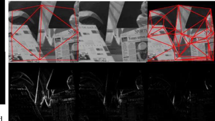
Next, the algorithm is tested on “Venus” [10] (Figure 3), a data for which only the uncalibrated cameras are known. The process, as depicted in Figure 5, starts with an 8-point reconstruction, and the distortion converges at 30 vertices. The errors due to the automatic localization of the corners and matching increase the residual error.

A final experiment is conducted on “Cliff”, a real video sequence, acquired from broadcast TV content (Fig.6), thus neither the scene geometry, nor the cameras are known. The process, presented in Figure 7, starts with an 8-point mesh, and the distortion converges at 50 vertices. As expected, errors in the cameras and the geometry further degrade the results, when compared to “Cube” and “Venus”. The lack of features in some parts of the scene prevents their

representation in the scene model and causes the black regions in Figure 6.

The number of iterations required for the convergence of the non-linear refinement stage, presented in Table 1, decreases with the increasing complexity of the geometry. This is due to the fact the local minima generated in more complex cases cause early termination, and reduce the effectiveness of this stage.

5. CONCLUSION

In this paper, a piecewise planar 3D reconstruction algorithm is proposed. The algorithm seeks a favorable point on rate-distortion curve by refining an initial mesh through the addition of new vertices, whose locations are determined by the prediction error. The experiments indicate that the proposed algorithm can yield efficient representations, thus it is an important step towards rate-distortion optimal 3D reconstruction for multi-view compression. However, in applications in which camera, structure or both should be estimated from the sequence, the algorithm requires accurate estimates of these parameters, in order to achieve satisfactory results.

6. REFERENCES

[1] A. Alatan and L. Onural, “Estimation of Depth Fields Suitable for Video Compression based on 3D Structure and Motion of Objects,'' IEEE Trans. on Image Proc., vol. 5, no. 6, pp.904-908, June 1998.

[2] A. Bartoli, P. Sturm, and R. Horaud, “A Projective Framework for Structure and Motion Recovery from Two Views of a Piecewise Planar Scene”, Technical Report RR-4970, INRIA, 2000.

[3] K. Schindler, “Spatial Subdivision for Piecewise Planar Object Reconstruction”, Proc. of SPIE and IS&T Electronic Imaging-Videometrics VIII, pp. 194-201, St. Clara, CA, 2003. [4] R. Musin, “Properties of the Delaunay Triangulation”, in

Proc. of 13th Annual Symposium on Computational Geometry, pp. 424-426, 1997.

[5] H. Hoppe, T. DeRose, T. Duchamp, J. McDonald, W. Stuetzle, “Surface Reconstruction from Unorganized Points”, ACM SIGGRAPH, pp. 71-78, 1992.

[6] D. D. Morris, and T. Kanade, “Image Consistent Surface Triangulation”, in Proc. of CVPR, pp. 332-338, 2000. [7] G. Vogiatzis, P. Torr, and R. Cipolla, “Bayesian Stochastic

Mesh Optimization for 3D Reconstruction”, in Proc. of BMVC, vol.2, pp. 711-718, 2003.

[8] J. H. Park, and H. W. Park, “A Mesh Based Disparity Representation Method for View Interpolation and Stereo Image Compression”, IEEE Trans. on Image Processing, Vol.15, No.7, pp. 1751-1762, 2006.

[9] “3D Time Varying Scene Representation Technologies: A Survey”, 3DTV NoE Technical Report, 2005.

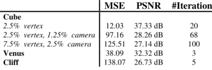
MSE PSNR #Iterations Cube 2.5% vertex 12.03 37.33 dB 20 2.5% vertex, 1.25% camera 97.16 28.26 dB 68 7.5% vertex, 2.5% camera 125.51 27.14 dB 100 Venus 38.09 32.32 dB 3 Cliff 138.07 26.73 dB 5

Table 1: Final distortion after non-linear optimization

[10] http://cat.middlebury.edu/stereo/data.html

[11] Hartley R., Zisserman A., Multiple View Geometry in

Computer Vision, Cambridge University Press, Cambirdge, 2003.

Figure 2: “Cube”, 7.5% perturbation in geometry, 2.5%

perturbation in cameras. Top row,left to right: Reference and target and predicted frames. Bottom row, left to right: Initial error, error before linear refinement, error after non-linear refinement. Reference frame is overlayed with the projection of the initial mesh, and predicted frame, with the projection of the 12-vertex mesh

Figure 6: “Cliff”. Top row,left to right: Reference and target

and predicted frames. Bottom row, left to right: Initial error, error before non-linear refinement, error after non-linear refinement. Errors are scaled by 3 to enhance visibility. Reference frame is overlayed with the projection of the initial mesh, and predicted frame, with the projection of 50-vertex mesh MSE vs. # Vertices 0 50 100 150 200 250 0 10 20 30 40 50 60 70 80 90 # Vertices MS E

Figure 5: Rate-distortion plot for “Venus”.

MSE vs. # Vertices 0 50 100 150 200 250 300 350 400 0 50 100 150 200 250 300 350 400 450 # Vertices MS E

Figure 7: Rate-distortion plot for “Cliff”.

MSE vs. # Vertices 0 500 1000 1500 2000 2500 1 2 3 4 5 6 7 8 9 10 11 12 # Vertices MS E No noise Vertex 2.5% Vertex 2.5% Camera 1.25% Vertex 5% Camera 1.25% Vertex 7.5% Camera 2.5%

Figure 4: Rate-distortion plot for “Cube” at various noise levels.

Figure 3: “Venus” Top row,left to right: Reference and

target and predicted frames. Bottom row, left to right: Initial error, error before linear refinement, error after non-linear refinement. Errors are scaled by 3 to enhance visibility. Reference frame is overlayed with the projection of the initial mesh, and predicted frame, with the projection of the 30-vertex mesh