Novel methods in image halftoning

T í h i Z i r r - O f 'f Í ! ? ^ S ¿ T ^ "''.Г'^О "’J ‘Ъ 'ГУ/,С 1" і <^/с. Ό

NOVEL METHODS IN IMAGE HALFTONING

A THESIS

SUBMITTED TO THE DEPARTMENT OF ELECTRICAL AND ELECTRONICS ENGINEERING

AND THE INSTITUTE OF ENGINEERING AND SCIENCES OF BILKENT UNIVERSITY

IN PARTIAL FULFILLMENT OF THE REQUIREMENTS FOR THE DEGREE OF

MASTER OF SCIENCE

By

Gozde Bozkurt July 1998

1

2 s f

I certify that I have read this thesis and that in my opinion it is fully adequate,

in scope and in quality, as a thesis for the degree of Master of Science.

Prof. Dr. Ahmet Enis Çetin(Supervisor)

I certify that I have read this thesis and that in my opinion it is fully adequate,

in scope and in quality, as a thesis for the degree of Master of Science.

Assist. Prof. Dr. Orhan Ankan

I certify that I have read this thesis and that in my opinion it is fully adequate,

in scope and in quality, as a thesis for the degree of Master of Science.

Assoc. Prof. Dr. Billur Barshan

Approved for the Institute of Engineering and Sciences:

r £ t 2 n

Prof. Dr. Mehmet Baray 1 .

Director of Institute of Engineering and Sciences

A B S T R A C T

N O V E L M E T H O D S IN IM A G E H A L F T O N IN G

Gözde Bozkurt

M .S. in Electrical and Electronics Engineering Supervisor: Prof. Dr. Ahmet Enis Çetin

July 1998

Halftoning refers to the problem of rendering continuous-tone (contone) images on display and printing devices which are capable of reproducing only a limited number of colors. A new adaptive halftoning method using the adaptive QR- RLS algorithm is developed for error diffusion which is one of the halftoning techniques. Also, a diagonal scanning strategy to exploit the human visual system properties in processing the image is proposed. Simulation results on color images demonstrate the superior quality of the new method compared to the existing methods. Another problem studied in this thesis is inverse halfton­ ing which is the problem of recovering a contone image from a given halftoned image. A novel inverse halftoning method is developed for restoring a contone image from the halftoned image. A set theoretic formulation is used where sets are defined using the prior information about the problem. A new space domain projection is introduced assuming the halftoning is performed ,with er­ ror diffusion, and the error diffusion filter kernel is known. The space domain, frequency domain, and space-scale domain projections are used alternately to obtain a feasible solution for the inverse halftoning problem which does not have a unique solution. Simulation results for both grayscale and color images give good results, and demonstrate the effectiveness of the proposed inverse halftoning method.

Keywords·. Color image halftoning, error diffusion, adaptive error diffusion, image restoration, inverse halftoning, inverse error diffusion, projection onto convex sets (POCS).

Ö ZE T

Y E N İ İM G E Y A R IT O N L A M A Y Ö N T E M L E R İ

Gözde Bozkurt

Elektrik ve Elektronik Mühendisliği Bölümü Yüksek Lisans Tez Yöneticisi: Prof. Dr. Ahmet Enis Çetin

Temmuz 1998

Yantonlama, sürekli tonlu imgelerin sınırlı sayıda renk üreten basma ve gösterim cihazlarında üretilmesi problemidir. Bir yantonlama tekniği olan hata dağıtılmasında, uyarlanır QR-RLS algoritması kullanılarak yeni bir uyarlanır yantonlama yöntemi geliştirilmiştir. Ayrıca, imgeyi işlemede insan görme sis­ temi özelliklerini kullanan bir köşegen tarama stratejisi önerilmiştir. Renk­ li resimler üzerindeki benzetim sonuçları, önerilen yöntemin diğer yöntem­ lere göre yüksek kalitesini göstermiştir. Bu tezde çalışılan diğer bir prob­ lem, sürekli tonlu imgenin verilen yantonlu imgeden geri elde edilmesi prob­ lemi olan ters yantonlamadır. Yantonlu imgeden sürekli tonlu imge elde et­ mek için yeni bir ters yantonlama yöntemi geliştirilmiştir. Problem hakkında önceden bilinen bilgileri kullanarak tanımlanan kümelerle, küme teorisine

dayalı bir formülasyon kullanılmıştır. Yantonlamanm hata dağıtılması ile

yapıldığı, ve hata dağıtma süzgecinin bilindiği varsayılarak, yeni bir uzay tanım kümesi izdüşümü geliştirilmiştir. Uzay, sıklık, ve uzay-ölçek tanım kümeleri izdüşümleri kullanılarak tek bir çözümü olmayan ters yantonlama problemine bir olurlu çözüm elde edilmektedir. Gri ölçekli ve renkli imgelere önerilen yöntemin uygulanması, iyi sonuçlar vermiş, ve geçerliliğini göstermiştir.

Anahtar Kelimeler: Renkli imge yantonlama, hata dağıtma, uyarlanır hata dağıtma, imge geri getirme, ters yantonlama, ters hata dağıtma, dış bükey kümelere izdüşüm.

A C K N O W L E D G E M E N T

I gratefully thank my supervisor Prof. Dr. Enis Çetin for his supervision, guidance, and suggestions throughout the development of this thesis.

I would like to thank Assist. Prof. Dr. Orhan Arikan for his suggestions, encouragement, and valuable discussions, and Assoc. Prof. Dr. Billur Barshan, the members of my jury, for reading and commenting on the thesis.

It is a pleasure to express my special thanks to my mother, and father for their sincere love, support and encouragement.

Contents

1 INTRODUCTION

1

1.1 M otivation... 2

1.2 H alfton in g... 3

1.2.1 Dithering T ech niques... 4

1.2.2 Error Diffusion Techniques... 5

1.2.3 Optimization-based Halftoning T ech n iqu es... 8

1.2.4 Hybrid Schem es... 9

1.3 Inverse Halftoning... 10

1.4 Contribution and Scope 13

2 AN ADAPTIVE ERROR DIFFUSION METHOD

15

2.2 A New Adaptive Error D iffusion... 18

2.3 Simulation R e s u l t s ... 22

3 A SET THEORETIC INVERSE HALFTONING METHOD 44

3.1 B a ck g ro u n d ... 44

3.1.1 Set Theoretic F orm u lation... 45

3.2 Method 49

3.2.1 Space-Domain Projection 50

3.2.2 Frequency-Domain P r o je c t io n ... 53

3.2.3 Space-Scale Domain Projection 54

3.3 Simulation Results 56

3.3.1 Restoration of Grayscale Im ages... 56

3.3.2 Simulation Studies for Color Im ages... 61

4 CONCLUSIONS AND FUTURE WORK

92

APPENDICES

94

A CONVEXITY OF THE SETS USED IN SET THEORETIC

List of Figures

2.1 Block diagram of error diffusion method... 16

2.2 Error Diffusion Filter Masks; (a) Floyd-Steinberg, (b) Jarvis,

Judice and Ninke... 16

2.3 Diagonal Scanning: dots correspond to the current pixel, and

the L-shaped window contains the previous pixels... 18

2.4 Prediction of the quantization error... 19

2.5 QR Linear Combiner, Scalar Implementation. 21

2.6 QR Linear Combiner, Vector Implementation... 22

2.7 Original Sunset Image 28

2.8 Quantized Sunset Image (16 c o l o r s ) ... 28

2.9 Error-diffused Sunset Image with Floyd-Steinberg’s Method 28

2.10 Error-diffused Sunset Image with LMS ada p ta tion ... 29

2.11 Error-diffused Sunset Image with QR-RLS adaptation... 29

2.12 Error-diffused Sunset Image with LMS adaptation (diagonal scan) 30

2.13 Error-diffused Sunset Image with QR-RLS adaptation (diagonal s c a n ) ... 30

2.14 Comparison of the error spectra of a line of the Sunset image. 31

2.15 Comparison of the error spectra with raster scan and diagonal scan of a line of the Sunset image... 31

2.16 Comparison of the average error spectra over all lines of the Sunset image... 31

2.17 Original Peppers Im a ge... 32

2.18 Quantized Peppers Image (16 colors) 33

2.19 Error-diffused Peppers Image with Floyd-Steinberg’s Method . . 33

2.20 Error-diffused Peppers Image with LMS a d a p ta tio n ... 34

2.21 Error-diffused Peppers Image with QR-RLS a d a p ta tio n ... 34

2.22 Error-diffused Peppers Image with LMS adaptation (diagonal s c a n ) ... 35

2.23 Error-diffused Peppers Image with QR-RLS adaptation (diagonal s c a n ) ... 35

2.24 Comparison of the error spectra of a line of the Peppers image. . 36

2.25 Comparison of the error spectra with raster scan and diagonal scan of a line of the Peppers image... 36

2.26 Comparison of the average error spectra over all lines of the

Peppers image. 36

2.27 Original Minnesota I m a g e ... 37

2.28 Quantized Minnesota Image (16 c o lo r s ) ... 37

2.29 Error-diffused Minnesota Image with Floyd-Steinberg’s method (16 c o lo r s ) ... 37

2.31 Error-diffused Minnesota Image with QR-RLS adaptation (16 c o l o r s ) ... 38

2.32 Error-diffused Minnesota Image with LMS adaptation (diagonal

scan, 16 colors) 39

2.33 Error-diffused Minnesota Image with QR-RLS adaptation (di­ agonal scan, 16 c o l o r s ) ... 39

2.34 Quantized Minnesota Image (8 colors) 40

2.35 Error-diffused Minnesota Image with Floyd-Steinberg’s method

(8 colors) 40

2.36 Error-diffused Minnesota Image with LMS adaptation (8 colors) 41

2.37 Error-diffused Minnesota Image with LMS adaptation (diagonal scan, 8 c o lo r s ) ... 41

2.38 Error-diffused Minnesota Image with QR-RLS adaptation (8 col­ ors) ... 42

2.39 Error-diffused Minnesota Image with QR-RLS adaptation (di­ agonal scan, 8 c o lo r s )... 42

2.40 Comparison of the error spectra of a line of the Minnesota image. 43

2.41 Comparison of the error spectra with raster scan and diagonal scan of a line of the Minnesota image... 43

2.42 Comparison of the average error spectra over all lines of the Minnesota image... 43

3.1 Relaxed projection onto C ... 47

3.2 Block diagram of error diffusion method... 50

3.4 Block diagram of the wavelet-based inverse halftoning scheme in [37]... 55

3.5 Inverse halftoning using the method in [37] with our method. . . 60

3.6 Original Peppers Image. 63

3.7 Peppers Image error diffused to 1 bit/pixel by Floyd-Steingberg’s Method... 63

3.8 Result of the first iteration in Table 3.1. 64

3.9 Result of three set of iterations in Table 3.1... 64

3.10 Zoomed sections from the first and last estimates in Table 3.1. . 65

3.11 Original Lena Image... 67

3.12 Lena Image error diffused to 1 bit/pixel by Floyd-Steingberg’s Method... 68

3.13 Result of the first iteration in Table 3.4. 69

3.14 Result of three set of iterations in Table 3.4... 69

3.15 Result of three set of iterations in Table 3.5... 70

3.16 Zoomed sections from the first and last estimates in Table 3.4. . 70

3.17 Peppers Image error diffused to 2 bits/pixel by Floyd-Steingberg’s Method... 72

3.18 Result of the first iteration in Table 3.7. 73

3.19 Result of two set of iterations in Table 3.7... 74

3.20 Lena Image error diffused to 2 bits/pixel by Floyd-Steingberg’s Method... 77

3.22 Result of two set of iterations in Table 3.8... 78

3.23 Result of three set of iterations in Table 3.9... 79

3.24 Result of the one set of iteration in Table 3.10... 80

3.25 Result of the two sets of iterations in Table 3.13... 81

3.26 Result of the one set of iteration in Table 3.12... 82

3.27 Lena Image error diffused to 1 bit/pixel by QR-RLS adaptation. 83 3.28 Result of the first iteration in Table 3.15... 84

3.29 Result of three set of iterations in Table 3.15. 85 3.30 Result of the first iteration in Table 3.16... 87

3.31 Result of two set of iterations in Table 3.16. 88 3.32 Result of the first iteration in Table 3.18... 89

3.33 Result of two set of iterations in Table 3.18. 89 3.34 Result of the first iteration in Table 3.17... 90

3.35 Result of two set of iterations in Table 3.17. 90

3.36 Result of the first set of iteration in Table 3.19. 91

3.37 Result of two set of iterations in Table 3.19. 91

List of Tables

3.1 The PSNR values after each iteration for the halftoned 1 bit

Peppers image. F (S) letter in the first column corresponds to the Frequency (Space) projection, (e.g. Sl-2 means 2” ^^ itera­

tion in the spatial projection) Type denotes the type of the

projection... 66

3.2 The PSNR values after each iteration for the halftoned 1 bit

Peppers image. F (S) letter in the first column corresponds to the Frequency (Space) projection, (e.g. Sl-2 means 2” ^^ itera­ tion in the R* spatial projection) Type denotes the type of the projection... 67

3.3 The PSNR values after each iteration for the halftoned 1 bit Peppers image. F (S) letter in the first column corresponds to the Frequency (Space) projection, (e.g. Sl-2 means 2” '^ itera­

tion in the spatial projection) Type denotes the type of the

projection... 68

3.4 The PSNR values after each iteration for the halftoned 1 bit Lena image. F (S) letter in the first column corresponds to the

Frequency (Space) projection, (e.g. Sl-2 means iteration in

3.5

3.6

3.7

3.8

3.9

The PSNR values after each iteration for the halftoned 1 bit Lena image. F (S) letter in the first column corresponds to the Frequency (Space) projection, (e.g. Sl-2 means 2"'^ iteration in

the spatial projection) Type denotes the type of the projection. 72

Comparison of inverse halftoning methods in [36], and our method for the Lena Image. The (GLPF, LPF, SVD) denotes

the type of frequency-domain projection 73

The PSNR values after each iteration for the halftoned 2 bit Peppers image. F (S) letter in the first column corresponds to

the Frequency (Space) projection, (e.g. Sl-2 means 2^^ itera­

tion in the spatial projection) Type denotes the type of the

projection... 75

The PSNR values after each iteration for the halftoned 2 bit Lena image. F (S) letter in the first column corresponds to the Frequency (Space) projection, (e.g. Sl-2 means 2"^^ iteration in the P* spatial projection) Type denotes the type of the projection. 76

The PSNR values after each iteration for the halftoned 2 bit Lena image. F (S) letter in the first column corresponds to the Frequency (Space) projection, (e.g. Sl-2 means 2” *^ iteration in the P ‘ spatial projection) Type denotes the type of the projection. 77

3.10 The PSNR values after each iteration for the Lena image. SS (S) letter in the first column corresponds to the Space-Scale (Space) projection, (e.g. Sl-2 means 2"^^ iteration in the P*

spatial projection) Type denotes the type of the projection. . . . 79

3.11 The PSNR values after each iteration for the Lena image. SS (S) letter in the first column corresponds to the Space-Scale (Space) projection, (e.g. Sl-2 means 2"·'^ iteration in the P ' spatial projection) Type denotes the type of the projection. . . . 80

83

84 3.12 The PSNR values after each iteration for the Peppers image.

SS (S) letter in the first column corresponds to the Space-Scale (Space) projection, (e.g. Sl-2 means 2” ^^ iteration in the

spatial projection) Type denotes the type of the projection. . . . 82

3.13 The PSNR values after each iteration for the Lena image. SS (S) letter in the first column corresponds to the Space-Scale (Space) projection, (e.g. Sl-2 means 2” ^^ iteration in the R* spatial projection) Type denotes the type of the projection. . .

3.14 Comparison of inverse halftoning methods. All methods assume the error diffusion kernel is known.

3.15 The PSNR values after each iteration for the Lena image error diffused with QR-RLS adaptation to 1 bit/pixel. F (S) letter in the first column corresponds to the Frequency (Space) projec­ tion. (e.g. Sl-2 means 2” *^ iteration in the 1®‘ spatial projection)

Type denotes the type of the projection. 85

3.16 The PSNR values after each iteration for the color Peppers image error diffused to 4 bits/pixel. F (S) letter in the first column corresponds to the Frequency (Space) projection, (e.g. Sl-2 means 2"^^ iteration in the R* spatial projection) Type denotes the type of the projection... 86

3.17 The PSNR values after each iteration for the color Minnesota image error diffused to 4 bits/pixel. F (S) letter in the first column corresponds to the Frequency (Space) projection, (e.g. Sl-2 means 2” ^ iteration in the R'* spatial projection) Type de­ notes the type of the projection...

86

3.18 The PSNR values after each iteration for the luminance compo­ nent (Y) of the color Peppers image halftoned to 4 bits/pixel. F (S) letter in the first column corresponds to the Frequency (Space) projection, (e.g. Sl-2 means 2"^^ iteration in the 1 spatial projection) Type denotes the type of the projection. .

st

3.19 The PSNR values after each iteration for the luminance com­ ponent (Y) of the color Minnesota image error diffused to 4 bits/pixel. F (S) letter in the first column corresponds to the Frequency (Space) projection, (e.g. Sl-2 means 2"*^ iteration in the 1®* spatial projection) Type denotes the type of the projection. 88

Chapter 1

IN T R O D U C T IO N

Halftoning refers to the problem of rendering continuous-tone (contone) images on display and printing devices which are capable of reproducing only a limited number of colors. This reduction in the number of colors causes a highly visible degradation in the quality of the image that naturally contains thousands or millions of colors. As a common solution to this problem, halftoning techniques are used.

In this thesis, a new adaptive signal processing algorithm is employed in the method of error diffusion which is a widely used halftoning technique. Various space filling curves to define the order of processing in error diffusion exist in literature. In this thesis, a diagonal space filling curve to exploit the human visual system properties in processing the image is proposed. Simulation re­ sults on color images are presented to demonstrate the superior quality of the proposed method compared to the other methods.

Inverse halftoning is the problem of recovering a contone image from a given halftoned image. In this area, less research has been performed than halftoning. In this thesis, a novel inverse halftoning method is proposed to restore a contone image close to the original contone image. A set theoretic formulation is used where three sets are defined using the prior information about the problem. A new space domain projection is introduced assuming

the halftoning is performed with error diffusion, and the error diffusion filter kernel is known. The space domain, frequency domain, and space-scale domain projections are used alternately to obtain a feasible solution for the inverse halftoning problem which does not have a unique solution. Simulation results for both grayscale and color images are presented.

In this Chapter, a survey on halftoning and inverse halftoning literature is given. Finally, the contribution and scope of this thesis is presented.

1.1

Motivation

Increasing demand for digital display of images on any of a wide variety of devices, and the increasing use of halftone printers to make hard copy outputs are given as the motivation for the research that resulted in part of this thesis.

In most computer color displays, the images are stored in a video memory. There, usually they are first recorded as full color images, where each color pixel is represented by 8 or 12 bits for each of the three channels. However, supporting storage of these full color images requires a high cost for high speed video memory. Many color display devices therefore reduce memory require­ ments by allocating 8,12, or 16 bits of video memory for each color pixel, thus allowing 2^, 2^^, or 2^® number of colors to be displayed simultaneously. Then, a palletized image which contains only colors from a limited palette, is stored in video memory and rapidly displayed using look-up tables [1]. However, di­ rect quantization from a very large set of colors to a very limited set of colors produces contouring effects in the output image. To prevent this problem, halftoning methods are used.

Printing devices are classified as contone and halftone printers [1]. Pho­

tography is the best known process that produces contone images. Using

photochemical methods which mimic photography, contone printing can be realized [1]. However, since they are rather expensive, most printers used are

halftoning technologies. This technology creates an extremely large number of pictorial images daily [2].

Color output devices such as halftone color printers and palette-based dis­ plays are capable of producing only a limited number of colors, whereas the human eye can distinguish around ten million colors under optimal viewing conditions [1]. Therefore, today, digital halftoning plays a key role in almost every discipline that involves printing and displaying.

Halftoning has enormous practical value, and a considerable amount of re­ search has been performed in this area. The inverse problem of reconstructing a contone image from its halftone version has also a large number of applications but much less research has been performed. This fact is the motivation for the research that resulted in the second part of this thesis. Contone images are needed instead of halftone in order to perform typical image processing tasks such as scaling, enhancement, tone correction, sharpening, decimation, inter­ polation, extrapolation, rehalftoning, compression, edge detection, recognition, linear or nonlinear filtering.

1.2

Halftoning

The eye perceives only a local spatial average of the color spots produced by a printing device, and is relatively insensitive to errors made in high frequen­ cies in an image [1]. Halftoning algorithms, therefore aim to preserve these local averages while forcing the errors between the contone image and the halftone image to high frequency regions. The existing halftoning techniques can be broadly classified as dithering techniques, error diffusion techniques, optimization-based halftoning techniques and hybrid techniques. An overview of literature in each of these classes is given next.

1.2.1

Dithering Techniques

Random dither, or white noise dithering is historically the first attempt to reduce the visible artifacts of direct quantization. The basic idea in dithering methods is thresholding each pixel value after adding noise to each pixel. It is also known as Roberts’ pseudo-noise technique, and it works by adding white noise to each pixel before quantization [3]. Roberts pointed out that dither does not increase the noise energy but simply redistributes the quantization noise to make it less visible. In frequency domain, the error in coarse quantizing a contone level is low in frequency and highly visible, whereas halftoning produces errors that are higher in frequency and therefore less visible.

The second class of dithering techniques employ dither matrices that quan­ tize the image by pixelwise thresholding. In conventional digital color halfton­ ing for printers, the image is decomposed into cyan, magenta, yellow, and black separations which are halftoned independently [1]. Black colorant is in­ troduced to produce denser blacks, reduce ink usage, and to conserve more expensive colorants. The halftoning for each separation is done by comparing each pixel value with a deterministic, spatially periodic dither array. Pixels for which the image exceeds the value in the corresponding dither matrix are turned on. Overlaying screens of color components with the same orientation causes the problem of registration. Some variation in the alignment of these color screens caused by the mechanical systems used in movement of the re­ production medium produces an artifact called moire patterns [1]. The effect is manifested as color shifts. Therefore, rotated screens are used where the rotation angle is chosen so as to minimize the occurrence and visibility of low frequency interference moire patterns. The most visible black screen is oriented along a 45° angle, along which the eye is least sensitive. The yellow, magenta, and cyan screens are located along 0°, 15°, and 75°, respectively [4].

Ordered dither algorithms are generally classified as two types: clustered- dot dither, and dispersed dot dither [5]. In clustered dot dither, the lower threshold values are centered in the pattern, causing a central dot that in­ creases in size as the pixel value increases. In the dither matrix, the thresholds

pixels. As the image value increases, the size of the clustered dots increases. In dispersed dot dither, the lower threshold values are scattered throughout the pattern, causing small dispersed dots that increase in number as the signal value increases [6].

Clustered dot patterns are insensitive to most printing distortions such as dot overlap, ink spreading, and reproduce well on printers that are incapable of reproducing isolated pixels. Therefore rotated clustered dot dithering is widely used for color printing. However, when the image is to be produced on a device that can successfully display every isolated pixel, the preferred choice is dispersed dot dither halftoning which maximizes the use of resolution [5]. For displays, alternate dither matrices that produce dispersed dots with greater spatial resolution are applied.

The ordered dithering techniques are attractive in the sense that they are very simple to implement, and computationally inexpensive because they re­ quire pixelwise operations. However, the major disadvantage of dithering is that it gives rise to regular error patterns due to the regular pattern of the noise introduced at different pixel locations.

1.2.2

Error Diffusion Techniques

The problems of moire patterns and color shifts created by misregistration of color screens in ordered dither is relatively eliminated by the error diffu­ sion algorithm, that is first introduced by Floyd and Steinberg [7], which re­ quires neighborhood operations. They proposed an algorithm which works by distributing the quantization error of the current pixel to neighboring pixels. Typically, at each pixel, the weighted sum of previous quantization errors is added to the current pixel, and the corrected sum is quantized to produce the output pixel. These weights form an error diffusion filter. The error diffusion aims to preserve the local average value of the image, therefore a unity gain lowpass finite impulse response (FIR) filter is used for distributing the error.

Error diffusion was first developed for grayscale images. For color images, error diffusion can be applied to each color component independently, which is

called scalar error diffusion, or as in [8], a color pixel can be error diffused in a vectorized manner.

Error diffusion works by shaping the error spectrum. In this method, the error is concentrated in high frequencies. This is suitable to the human eye which is less sensitive to high frequencies. Ulichney [5] proposed an error diffusion filter with randomized weighting coefficients to shape the display error spectrum to have mostly high frequency content, named as Blue Noise. He examined the spectral characteristics of the output error, and demonstrated that blue noise is less noticeable to the human eye than errors compared to the white power spectrum.

Error diffusion technique is still an active area of research. Variations on this technique are employed by many researchers.

Some directional artifacts seen in error diffusion are due largely to the traditional raster of processing [5]. Previous approaches for improving error diffusion employed various choices of space filling curves to define the order of processing, such as serpentine curves [5], Peano curves [9], random space filling curves [10]. In [10], purpose of randomness is to erase regular patterns arising usually in uniform intensity image regions. A disadvantage of this method is large memory consumption which is overcome by performing the halftoning for blocks of the image separately. Witten and Neal [9] used an error filter with one deterministic weight, and processed the image on a Peano curve.

In [11], error diffusion is modified by incorporating a color printer model that accounts for dot overlap distortion in printers. A human visual system model in the form of its Modulation Transfer Function (MTF) is incorporated into error diffusion in [12].

In contrast to deterministic error filter kernels, some recent research em­ ployed dynamically adjusting the error filter kernel using adaptive signal pro­ cessing techniques. Akarun, Yardımcı, and Çetin [8] have used a vectorized error diffusion approach, and updated the error diffusion filter coefficients adaptively. Wong [13] minimizes a local frequency-weighted error criterion

error diffusion algorithm to enable rendition at several resolutions which can be useful for progressive transmission.

Sequential nature of the error diffusion technique means that the errors get propagated in the direction the image is scanned, which can result in subtle artifacts. An algorithm in which the errors are diffused isotropically in all directions would be preferred.

For single pass processing of the image, error diffusion filter kernel is causal which implies that the filter is asymmetric. This asymmetry causes visible low frequency wormlike artifacts in binary error diffusion. Symmetric error diffusion neural networks have been proposed for gray scale images [15]. An all optical implementation of the symmetric error diffusion algorithm is given in [16]. One of the advantages of this implementation is its reduced computational complexity, and storage requirements, and high speed.

To allow usage of a non-causal error filter, a multi-pass error diffusion is proposed in [17], where the quantization error of one iteration (pass) is collected and used during the next iteration as quantization error of the future pixels. The error filter in this case is preferably chosen as a zero-phase filter so that feedback is added to the input image without affecting the phase to retain sharp edges. The disadvantage of this algorithm is its iterative nature.

Kolpatzik and Bouman [18] developed an optimization criterion for the design of an error diffusion filter, based on a model for the human visual system to include the effects of the monitor modulation function and human visual modulation transfer function combining the models in [6]. They also developed a locally dithered error diffusion algorithm combining the idea in random dither and error diffusion.

A fuzzy error diffusion method for color images is presented in [19] which makes use of membership functions indicating the location of a pixel with respect to each quantization color. This information is used to control the amount of error to be spread thus preventing the accumulation of errors.

Another modification to error diffusion of grayscale images proposed in [20] is introducing an input dependent threshold into the process to decrease or increase edge enhancement in the algorithm.

Most of the error diffusion methods existing in the literature are developed for halftoning of grayscale images. Only a few of the methods mentioned are proposed for color images where most are not efficient in producing a high quality color image output. Another disadvantage of these color error diffusion methods is their substantially high computational complexity.

1.2.3

Optimization-based Halftoning Techniques

The problem of halftoning can be formulated as an optimization problem that minimizes an error metric between the continuous tone original image and its halftone version. These techniques can be referred as optimization-based halftoning techniques which are iterative, and requires significantly more com­ putation than error diffusion based techniques, and ordered dither techniques. In this approach, the halftoning problem is posed as an optimization prob­ lem which maximizes the visual similarity between the original image and its halftone version.

In these methods, a distortion measure is defined, and some methods em­ ploy visual models or printer models in the definition of these measures. There­ fore, they are also referred as model-based halftoning techniques. Pappas [21] included both a printer model and a visual model. The simple eye model in [22] includes a memoryless nonlinearity followed by a filter which is chosen as the MTF referring to the spatial frequency sensitivity of the eye [23]. An optimal halftone image is found by minimizing the squared error between the output of the cascade of the printer and visual models in response to the halftone image and the output of the visual models in response to the original contone image. Two dimensional least-squares solution is obtained by iterative optimization techniques. A distortion measure in the frequency-domain, frequency weighted

on neural networks is suggested in [15]. Both a space-domain distortion mea­ sure and a frequency-domain distortion measure are proposed in [24], where the minimization procedure is performed blockwise in the image. In frequency- domain optimization, the weighting function is the MTF proposed in [23].

Similarly, an error metric related to the total generated error between the contone and halftone images is defined in [25]. The total error is filtered with contrast sensitivity function describing the visibility of signals as a function of the spatial frequency because the errors which are not visible are of no interest. A descent-type algorithm, and a simulated annealing algorithm are used for the optimization problem in [25]. Usage of genetic algorithms is proposed in [26] for optimization-based halftoning in a similar way.

Disadvantages of optimization-based methods for halftoning is that there are many local optima, the methods are iterative, and they require substantially high computational power. For color images, processing requirements further increase.

1.2.4

Hybrid Schemes

Hybrid schemes that combine different aspects of halftoning methods are pro­ posed in the literature.

Blue noise halftoning that combines the speed of dithering techniques with the quality of error diffusion techniques is the application of large dither ma­ trices produced for obtaining blue noise characteristics [27]. For color images, independent blue noise masks are used for each color component.

A number of researchers considered the problem of selecting an optimal color palette and the optimal mapping of each pixel of the image to a color from the palette in a unified manner. Orchard and Bouman [28] proposed a new error diffusion algorithm using an image specific color palette having a binary tree structure for efficient implementation. Similarly, in [29,30], dithering process is embedded in the quantization process. In [29], the cluster splitting strategy of [28] is modified at the leaves so that a pair of leaves after the split are

displaced in opposite directions to span a wider color space. In [30], palette colors in color space and color pixels in the color image are alternately updated. At each pixel, the palette color to which the pixel belongs is updated according to the competitive learning rule. Afterwards, error diffusion step is performed.

Halftoning algorithms based on multiresolution, pyramidal structure, for grayscale halftoning are proposed in [31,32]. In [31], at each pyramid level, the output binarized image is compared with the original grayscale image over a successively larger window of pixels, and some binary pixels are modified in order to reduce a weighted averaged error. Similarly, a multiscale error diffusion is proposed in [32] where the algorithm begins with the lowest resolution image at the top of the image pyramid, and proceeds by always selecting the quadrant with the highest average intensity.

1.3

Inverse Halftoning

Inverse halftoning is the problem of recovering a contone image from a given halftone image. This inverse problem can be thought as a restoration problem or a denoising problem since halftoning can be considered as a process that degrades the original image by introducing noise into it. Halftoning is a many- to-one mapping, therefore inverse halftoning problem does not a have a unique solution. Research in this area is considerably less than that is done for forward halftoning.

The existing inverse halftoning methods employ space-domain operations, frequency-domain operations, or both, or only space-scale domain operations. Literature on inverse halftoning contains research only for recovering a gray­ scale image from its binary halftone version. We give an overview of these methods next.

The simplest approach is lowpass filtering the halftone image to remove the high-frequency components. Since in error-diffused images, the errors are generally concentrated in the high frequencies, this approach seems reason­ able. Different lowpass filters have been used such as halfband lowpass in [33],

Gaussian lowpass and lowpass filtering based on singular value decomposition (SVD) [36]. However, lowpass filtering alone does not work well since this also destroys high-frequency information of the original image. This approach corresponds to ignoring the spatial constraints, and enforcing only frequency constraints.

A projection algorithm, which is essentially an error diflfusion with an addi­ tional inverse quantization step is proposed in [33]. Error diffusion is performed at each pixel starting with an approximation of the contone image, e.g., lowpass filtered version of the halftone image. The input pixel is adjusted so that the corrected pixel value at the input of the quantizer is quantized to the desired halftone value at the output. This projection in inverse quantization process is performed by maximum a posteriori probability (MAP) projection. A sim­ ilar method [34], based on a MAP estimator is proposed where a constrained optimization is solved using iterative techniques.

The method of Projection Onto Convex Sets (POCS) is used in [35, 36] where information known about the problem is expressed in the form of two constraint sets. Space-domain projection using the first constraint set, then frequency-domain projection using the second constraint set, are performed alternately, to find an image invariant under both. The first set is the set of all contone images which when halftoned give the desired halftone image, the second is the set of all images bandlimited to a certain band. The method in [35] is designed for recovering a contone image from an image halftoned with ordered dithering method. The frequency-domain projection is performed with lowpass filtering, and the space-domain projection is performed with making the minimum change necessary to each image pixel after comparison with the screen function.

Another method using the idea of POCS to reconstruct images from a X] A- based error diffused image, is proposed in [36]. A linear SVD based transform or a linear Gaussian filtering are used for frequency-domain projection. For the space-domain projection, they define a computational procedure for error diffusion by slightly modifying the error diffusion to reduce the complexity of their reconstruction algorithm. Using this, they propose a matrix space- domain description of the error diffusion encoder. However, the computational cost of the projection is very high because the algorithm turns out to be a

linearly constrained Quadratic Programming (QP) problem that tries to solve

512 X 512 matrix equations for an image of this size. They suggested solving

this problem by solving a number of QP subproblems of size Lq p, i.e., size of

the blocks, rather than solving one QP problem of size N'^.

In these techniques, the halftoning process is assumed to be known a priori. In case of ordered dither halftone images, an algorithm to estimate the screen function is proposed in [35]. Similarly, for error-diffused images, Wong [33] suggested a method to estimate the error diffusion kernel posing the problem as a system identification problem encountered in adaptive signal processing.

Xiong, Orchard, and Ramchandran [37] proposed an inverse halftoning

scheme using wavelets. The idea behind the wavelet decomposition of a

halftone image is to selectively choose useful information from each subband. This approach can be considered as a space-scale domain method. An explicit edge detection based on cross-scale correlation of the highpass wavelet images is done to perform spatially varying filtering of the halftone image. In this way, background halftoning noise is removed while important edge information is preserved in the bandpass bands. Furthermore, no a priori knowledge about the halftoning process is assumed.

Another wavelet-based inverse halftoning method is proposed in [38], where after subband decomposition of the halftone image, halftone noise in the sub­ bands is eliminated by spatial and frequency selective processing. Frequency selective processing corresponds to interband operations, and comparison of the magnitudes of the coefficients at different resolution levels but the same spatial location, then clipping some coefficient values accordingly. Spatial pro­ cessing corresponds to intraband filtering, i.e., oriented filtering tailored for each subband to preserve edges along its orientation.

In [39], a simple table-lookup method referred as a nonlinear decoder to convert error-diffused images back to the grayscale domain is implemented. Blocks of size 3 x 3 are used as an index into a table consisting of 512 distinct binary patterns. This look-up table is built by calculating an output gray value for each index (3 x 3) in the training sequence. Then each halftoned pixel is decoded based on its 3 x 3 neighborhood which gives the grayscale output from the table. This method is simple, however it needs a training phase to obtain

the look-up table. Furthermore, the reconstructed image quality is relatively lower.

1.4

Contribution and Scope

The first contribution of the thesis is the introduction of a new adaptive error diffusion method for color images. A rotation based Recursive Least Squares algorithm is used in the prediction where the error diffusion filter coefficients are updated adaptively. Both scalar and vector implementations of the pro­ posed method is developed. The scalar implementation processes each color component of the color image separately whereas the vector implementation uses all three color components in the prediction of each color component. Also a diagonal scan is used in processing the image to exploit the relative insen­ sitivity of the human visual system to diagonal orientations. The proposed method produces high quality halftone images with a very limited number of colors.

The second contribution of the thesis is the introduction of a set theoretic inverse halftoning method which restores the continuous tone image back from its halftone version. A new space-domain projection is proposed which defines a set for each pixel, and the projection is performed at each pixel using the a priori information that the halftoning is performed with the error diffusion method, and the error diffusion filter kernel is known. In addition, frequency and space- scale domain projections are used alternately with the proposed space-domain projection to find a feasible solution for the inverse halftoning problem that has no unique solution. Furthermore, the space-domain projection is extended for the case of multilevel error diflPusion encoding. This extension is in turn used for restoration of color images from their halftoned versions. The proposed inverse halftoning for color images may be viewed as a first attempt in this area.

Chapter 2 introduces the new adaptive error diffusion method that results into higher quality output images than that of Floyd-Steinberg’s method and

the error diffusion with Least Mean Square adaptation. Extensive simulation results are given to show the performance of the proposed method.

Chapter 3 introduces the proposed inverse halftoning method with a new space-domain projection. The simulation results of the proposed method is compared with those of the state-of-the-art inverse halftoning methods existing in the literature, based on their Peak Signal-to-Noise-Ratio’s.

Chapter 2

A N A D A P T IV E E R R O R

D IF F U SIO N M E T H O D

In this chapter, a new error diffusion method is presented in which the adaptive Recursive Least Squares (RLS) algorithm is used for prediction. Also, a diago­ nal scan is used in processing the image to take advantage of the human visual system. The simulation results of the proposed method is compared with that of the Floyd-Steinberg’s method, and the adaptive error diffusion with LMS al­ gorithm both with raster scan and diagonal scan of the image. The simulation studies show the superiority of the proposed adaptive error diffusion method.

2.1

Diagonal Error Diffusion

Block diagram of the standard error diffusion technique is given in Figure 2.1. Usually, the image is processed in a raster scan fashion, and each input color pixel x ( s i , S2) is a

3 X 1

(si,S

)

where M is the number of horizontal pixels in the image. The current pixel

X (s) together with the diffused error is quantized. The resultant image y ( s )

is the dithered image.

Here, Q is the quantizer, and h is the error diffusion filter. Some well-

known error diffusion filter masks [7,40] are shown in Figure 2.2 where · denotes the origin. These masks determine the support of the error diffusion filter. A common characteristic of these filters is that they are causal, i.e. their region of support is wedge-like to ensure that these filters can be applied in a sequential manner [41]. The filter coefficients are deterministic, lowpass in nature, and add up to 1 so that errors are neither amplified nor reduced.

.5 3

(— )_{16 7}

Floyd - Steinberg

1 3 5 3 1

3 5 7 5 3

Jarvis, Jiidice and Ninke

Figure 2.2: Error Diffusion Filter Masks: (a) Floyd-Steinberg, (b) Jarvis, Ju- dice and Ninke.

A weighted sum of the previous quantization errors in the window, and the current pixel x (s) are added to form u (s), and this value is quantized to obtain the dithered pixel value as follows:

u{ s ) — x { s ) + " ^ h { s — k)e (k) k<s e (s) ^ u ( s ) - y (s) y ( s ) = Q (u (s ))

(

.

)

2

2

where k < s corresponds to a causal error diffusion mask, and e (s) is the quantization error. The error between the original input pixel and the output

pixel is defined as the output error, Soutis) = x (s) - y (s) which can be

expressed as

e out{s) = e (s) - h {s - k)e (k) (2.4)

k<s

Let the 2-D Discrete-Time Fourier Transform of eout(s) to be

E o ut i w) ^ ^ (2.5)

where w is the 1-D index for w = (wi,W2) for simplicity, and Z is the set of

all integers. From (2.4), the output error spectrum becomes

E out{w) ^ E {w)[I - H { w ) ]

₍

2

_.

6

₎

where H (w) is the frequency response of the error diffusion filter. If the

quantization error spectrum is white, the output error spectrum can be shaped by the ( I — I f (w)) filter. Since I f (w) is lowpass, ( f — H (w)) is a highpass filter. This is a favorable feature of the error diffusion algorithm because the human visual system is less sensitive to high frequency components in an image. Furthermore, the error diffusion filter coefficients sum to 1, i.e., f l {0) = 1.

This leads to E o«t(0) = 0, and implies that the mean value of the quantized

image is matched to the original image mean.

The raster scan used in error diffusion causes vertical or horizontal artifacts, and regular patterns that arise especially in uniform intensity regions. It is well- known that human visual system is less sensitive to diagonal errors compared to the vertical or horizontal errors. To take advantage of this fact we scanned the image diagonally. In this way, the error is diagonally diffused, and the resulting artifacts are less bothersome. Causal prediction windows shown in Figure 2.3 are used in the error diffusion algorithm. Here, we aim to break up the horizontal and vertical directionality of the possible error patterns, and force the accumulation of the error to be in diagonal orientation to which the human eye is less sensitive.

Figure 2.3: Diagonal Scanning: dots correspond to the current pixel, and the L-shaped window contains the previous pixels.

2.2

A New Adaptive Error Diffusion

The error diffusion filter pla.ys an important role in shaping the output error

spectrum. The error filter should be designed so that the output error, eout{s),

is the least noticeable to a human observer [18]. In contrast to deterministic error diffusion filters, recent algorithms use the optimum filter coefficients for a given image, or update the coefficients adaptively using Least Mean Square (LMS) type adaptive algorithms [8,13].

As in standard dithering, in error diffusion, the aim is decorrelate the quan­ tization noise, the difference between the input and output of the quantizer, from the input signal. This results into a whiter error spectrum, so the er­ rors are less visible and less disturbing for the observers. This requires the prediction of the quantization error of the current pixel from the previous quantization errors. The prediction aims to minimize the energy of the output error eout{s), as shown in Figure 2.4, as follows:

F;[))e„„,(5)]p] = F ;[)|x (s )- y (6 0 in .

This is equivalent to minimizing

B ( | | e W - E '> ( s - * ) e W l P ] .

k<s

(2.7)

(

2

8

Then the optimal filter coefficients are chosen as the miniraizer of (2.8). Dif­

ferentiating (2.8) with respect to h{ i), and setting the results to zero, the

following set of linear equations are obtained:

E[e (s)e'^(s - i)] = ^ (s - k)E[e (s)e^(s - i)], k<s

Figure 2.4: Prediction of the quantization error.

The error diffusion coefficients h can be obtained by solving the system

of equations in (2.9). An estimate of the covariance matrix E[e (s)e^(s· — i)]

can be obtained from the quantization error statistics of the image. However, since a typical image does not have stationary characteristics, this approach does not yield satisfactory results.

Considering the fact that the image signal characteristics are generally non- stationary, that is significant difference exists in the statistics of different re­ gions of the image, an adaptive algorithm is used in the minimization of the output error sequence. In this thesis, in order to achieve better prediction than the LMS algorithm which was used in some earlier work, we considered using an RLS-type adaptive algorithm. The LMS provides an approximate solution to the Least Squares(LS) problem that arise in many applications of signal processing. Two different classes of methods have been developed for solving these problems: the LMS is based on the gradient descent technique, and the RLS algorithm uses exponentially weighted LS criterion.

The RLS algorithm provides an exact solution of the LS problem at each time step. There are various RLS algorithms, where most widely used are the Fast RLS algorithms such as Fast Transversal filters(FTF) [42]. These RLS algorithms were preferred because they provide optimal weights at ev­ ery sample, are faster than LMS-based techniques in convergence, and can be numerically more stable. However in the fast RLS algorithm, the input data vector is updated by a shift at each time step, and in the case of error diffu­ sion, the L-shaped window contains the pixels used in the prediction where the data vector is altered by a 2-D shift. Therefore, fast RLS algorithms are not exactly suitable for a linear combiner implementation which is the prediction problem o f the current quantization error. Recently, LS problems are solved

using rotation-based methods, based on updating the QR-decomposition of the input data matrix. These rotation-based algorithms are more robust to low precision arithmetic that reduce the implementation costs whereas non­ rotation-based RLS algorithms may break down [43]. QR algorithms offer fast convergence behavior and better tracking ability. The QR-linear combiner is well suited for the prediction problem in error diffusion. The complexity of the QR-RLS adaptation is Order(A^^), where LMS adaptation has a complexity of

Order(A^). N is the number of pixels in the prediction window, which is chosen

as = 4 as in Floyd-Steinberg’s method. Therefore, the complexity of the

QR-RLS algorithm does not increase much.

The basic linear LS estimator is the linear combiner. The problem of pre­ diction of the quantization error in error diffusion can be implemented as QR- linear combiner. Using a linear combination of the previous quantization error signals, we want to estimate the desired signal e (s). The previous quantization errors e { s — i) are represented as e ¿(s). The estimate is e (s) = /i^ (s)ep (s),

where ep(s) = [e i ( s ) , ..., e denotes the A^ x 1 data vector and h{ s)

denotes the weight vector. The purpose of recursive LS estimation is to choose

h (s) so as to minimize the sum of exponentially weighted squared errors.

^ A* "“[e (m) - h'^\s)ep{rn)f (

2

10

m = l

The factor 0 A < 1 is called the forgetting factor. Its aim is to forget the data in the distant past to have a better tracking capability in a nonstationary environment.

The summary of the QR-RLS algorithm is given as follows;

R { 0 ) = V s i N,'i^i0) = 0 for s = 1 , 2 , . . . Q (s) v / X i 2 ( s - l ) V ^ r ( 5 - 1 ) ep(s) e(5) 0^’ 7 (5) = n<^os^i(s) i = l f { s) = f { s ) j { s ) R{ s) r ( s ) R-'^\s) O’^(s) f(s) N

h{ s) = h { s - l ) - g { s ) f { s )

A detailed discussion of the QR-RLS algorithm can be found in [43].

In the implementation of the QR-Linear combiner, the previous quantiza­ tion errors in the causal so-called half plane window are used as inputs, and the current quantization error is used as the desired signal. In the scalar

imple-Figure 2.5: QR Linear Combiner, Scalar Implementation.

mentation of the algorithm, the red, green and blue components of each pixel are processed separately by running three QR-RLS algorithms in parallel, each giving the output for each one of the color components red, green, blue, as shown in Figure 2.5. The number of pixels in the prediction window of each

color component is chosen as N — 4 in our implementations.

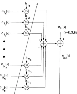
In the vector implementation, all three color components of the previous quantization errors are used in the prediction of the each component of the current quantization error, as in Figure 2.6. Again, three parallel QR-RLS algorithms are run for each of the color components. Here, the aim is to use the correlation among the color components. The number of pixels in the

prediction window, is chosen as = 12 in the vector implementation for each

color component.

Figure 2.6: QR Linear Combiner, Vector Implementation.

2.3

Simulation Results

In this section, we demonstrate the effectiveness of our error diffusion algorithm using three specially selected color images. To render the illusion of a color ramp, two photographs Sunset image, and Minnesota image are used. These images are good test images with slowly varying color regions. Third test image is the well-known Peppers image, which has both slowly varying regions, and sharp edges.

We implemented both the scalar and vector versions of the RLS-based adap­ tive error diffusion algorithm. We give the results of the scalar implementation. The results of the new algorithm is compared with that of the Floyd-Steinberg’s method, and the adaptive error diffusion with LMS algorithm both with raster scanning and diagonal scanning of the image. The quality measure for the re­ sulting images are the observer’s evaluations and whiteness comparison of the power spectrum of the quantization noise images.

The step size parameter n used in the implementation of the error diffusion with LMS is set to 0.95. A scaling coefficient of 0.9 is used which scales the error diffusion filter coefficients after each update. This means that all the errors are not fed back through this filter but only 90% of them are fed back to the input pixel before quantization. The forgetting factor parameter A in error diffusion with QR-RLS adaptation is chosen as 0.95 so that errors in the past are deemphasized, and the algorithm adapts to the local variations in the image.

VVe first give the simulation results for the Sunset image. The original image is shown in Figure 2.7, and the quantized image with median cut algorithm [44] to 16 colors is given in Figure 2.8, respectively. The quantized image shows the contouring effect very clearly in sea and sky regions, and false contours appearing because of the small number of available colors to represent these slowly varying color changing regions. The error diffused image with Floyd- Steinberg filter is shown in Figure 2.9 where contouring is a little improved, but the performance is poor in edge regions, i.e. the region where the sky and sea merge. The color impulses in the form of dots of a color emerging on a different colored background are visible. The error diffused images by adaptive algorithms LMS and QR-RLS adaptation using raster scan are shown in Fig­ ure 2.10 and Figure 2.11 respectively. The LMS-based adaptive error diffusion shows improvement when compared to that of the Floyd-Steinberg’s method in reducing the color impulses and the behavior in edge regions. However, as can be observed in Figure 2.11, nearly all of the problems of quantization and dithering are removed in QR-RLS based adaptive error diffusion. The sky and sea merge naturally, and the smooth transitions from one color to the next are successfully reproduced as in the original image. The error diffused im­ age by LMS adaptation with diagonal scan is shown in Figure 2.12. There’s slight improvement in removing the color impulses. The error diffused image by QR-RLS adaptation with diagonal scan is shown in Figure 2.13. These figures show that QR-RLS based adaptive error diffusion with both raster and diagonal processing are the most successful methods.

The areas of slowly varying regions, or areas of uniform intensity in an image are the most problematic regions for a halftoning algorithm. Therefore,

a good measure for the quality of a halftoning technique is the ability to render these areas. In this context, the proposed method gives the best result.

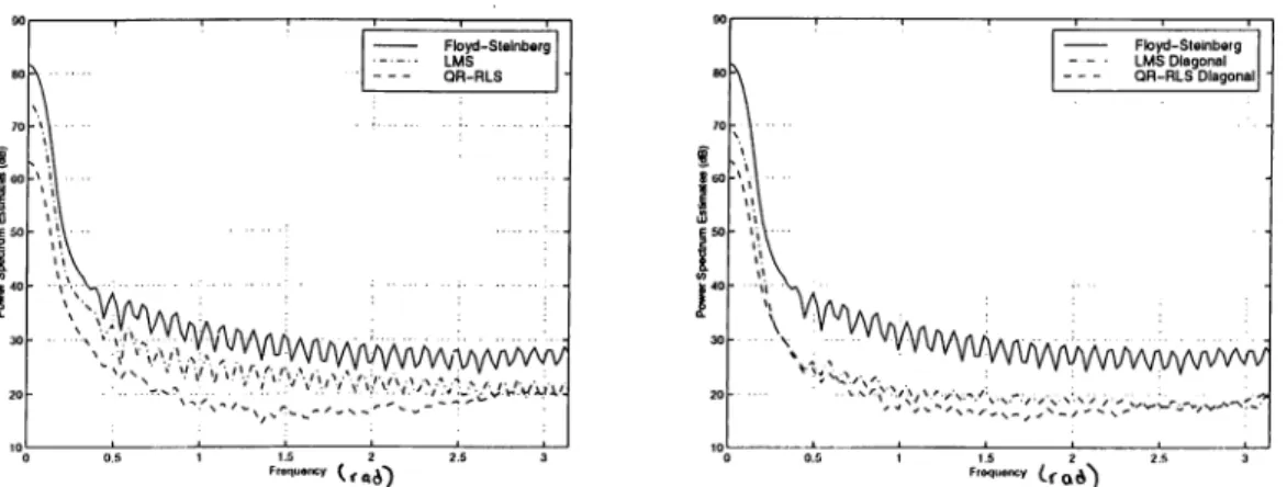
As a performance measure, we use the power spectra of the quantization er­ ror as pointed out in [18]. We estimate the power spectrum of the quantization error for the resulting images by Welch’s periodogram averaging method [45]. We compare estimates for LMS with raster scan, and with diagonal scan, QR- RLS with raster scan and diagonal scan, and Floyd-Steinberg’s method.

In Figure 2.14, the spectrum of the quantization errors in a horizontal line of the Sunset image is shown. Since it is difficult to plot 2-D spectrum, the spectrum of a line of the image is shown here. As can be observed from these plots, the power spectrum of the image error diffused by the QR-RLS adaptation method has not only the lowest energy but also the flattest response whereas the error diffusion with Floyd-Steinberg has the highest energy. The LMS-based method lies between the two curves. This experiment verifies the fact that QR-RLS based method produces the best results. Similar results are obtained for other lines of the image.

All three algorithms are compared also for diagonal scanning scheme in Figure 2.14. Floyd-Steinberg’s method always produces an error spectrum with the largest energy. The adaptive algorithms both reduce the energy with best performance corresponding to the QR-RLS based error diffusion method.

We also compare the power spectrum estimates for both types of order of processing the Sunset image, namely the raster and diagonal processing, as shown in Figure 2.15. In the first plot, we can see that the error spectrum for the error diffusion using LMS with diagonal scanning of the image is flatter than the one with raster processing, and has reduced energy.

The average error spectra over all lines of the image is shown in Figure 2.16. It is observed that the proposed method with QR-RLS adaptation shows the flattest response also for an average of the lines image. This verifies our obser­ vation that similar results are obtained for all lines of the image.

The simulation results for the well-known Peppers image are given next. The original Peppers image is shown in Figure 2.17, and the quantized ima,ge

to 16 colors with median cut algorithm is shown in Figure 2.18. False contours are clearly visible particularly on the green pepper in the middle because it has slowly varying color regions on its body from green to red and again to green and so on. This is again one of the problematic regions of the Peppers image. Figure 2.19 shows the image error diffused by Floyd-Steinberg’s method. White color impulses on the upper red pepper are observed. Actually, we can see that Floyd-Steinberg’s method produces very poor results in the edge regions which are smeared to each other. The color impulses are highly visible, and color shifts especially in the top region of the pepper in the middle is very disturbing. The Peppers image error diffused with LMS adaptation shown in Figure 2.20 shows better performance, and improves the behavior in edge regions. The color impulses are eliminated. However, the contouring effects in the mentioned problematic region are disturbing because the transition is not smooth. The resulting image error diffused with QR-RLS adaptation is shown in Figure 2.21. It is observed that this image shows the most superior performance among the error diffusion methods discussed so far. It is sharper and brighter, and the problematic region shows smooth transition for the slowly varying colors. The images for the adaptive error diffusion methods with diagonal scanning are given in Figure 2.22, and Figure 2.23. The image error diffused with QR-RLS adaptation gives the highest quality output.

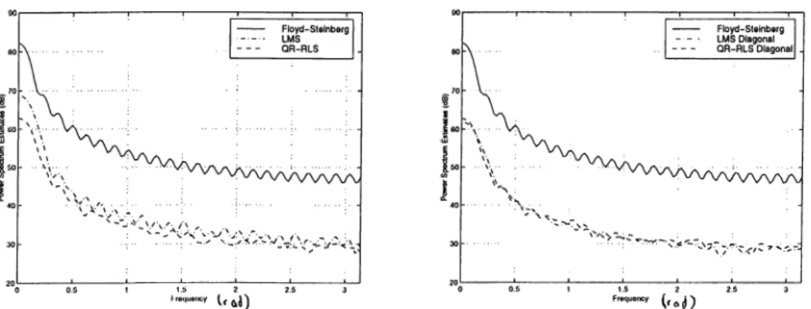
For the Peppers image, we also plot the error power spectra for the three algorithms in Figure 2.24. The performance of the adaptive methods for the raster scan is such that the method with QR-RLS gives the lowest energy and flattest response. The one with LMS gives the second lowest energy response. The Floyd-Steinberg’s method has the highest energy. For the diagonal scan, LMS shows improvement and has a lower energy error spectrum than that of the raster scan.

The error spectra for raster and diagonal scanning of both adaptive error diffusion methods are shown in Figure 2.25. The average of the error spectra over all lines of the image for the three methods is shown in Figure 2.26. There­ fore, on the overall response, the error spectra of the adaptive error diffusion method QR-RLS adaptation shows the flattest response.

The simulation results for the Minnesota image are given in the following. The original image in Figure 2.27 is quantized to 16 colors with the median