CO
2EMISSIONS, ENERGY CONSUMPTION AND ECONOMIC
GROWTH IN THE USA AND THE UNITED KINGDOM:
ARDL APPROACH
Hakan ÇETİNTAŞ*
ve Murat SARIKAYA**
Abstract
This study investigates the effects of energy consumption and the economic growth on the carbon dioxide emissions and causality in a multivariate model, which includes nuclear energy generation, foreign trade and urbanization variables, in the UK and the USA by employing data of 1960-2004. Cointegration test results support that there is a long-term relationship among the variables. While the economic growth in the UK has a positive effect on CO2 emissions in the short term and long term, the economic growth in
the USA does not affect CO2 emissions. In both countries, there is a positive relationship
between energy consumption and CO2 emissions and a negative relationship between
nuclear energy generation and CO2 emissions. There is a unidirectional causality from CO2
to economic growth in the UK and from energy consumption to CO2 emissions in the USA.
In both countries, we have detected no causal relationship between energy consumption and the economic growth.
Keywords: CO2, Growth, Energy Consumption, Causality
ABD ve İngiltere'de CO2 Emisyonu Enerji Tüketimi ve Ekonomik Büyüme: ARDL Yaklaşımı
Özet
Bu çalışmada 1960-2004 arasında İngiltere ve ABD'de karbon emisyonlarının ekonomik büyüme ve enerji tüketimi üzerindeki etkileri ve nükleer enerji üretimi, dış ticaret ve şehirleşme değişkenleri dahil çok değişkenli bir model çerçevesinde nedensellik ilişkileri araştırılmıştır. Koentegrasyon test sonuçları söz konusu değişkenler arasında uzun dönem bir ilişkinin varlığını doğrulamaktadır. İngiltere'de ekonomik büyüme kısa ve uzun dönemde CO2 emisyonları üzerinde pozitif bir etkiye sahipken ABD'de ekonomik büyümenin CO2 emisyonları üzerinde bir etkisi bulunmamaktadır. Her iki ülkede de enerji tüketimi ve CO2 emisyonları arasında pozitif bir ilişki, nükleer enerji üretimi ve CO2 emisyonları arasında negatif bir ilişki vardır. İngiltere'de CO2'den ekonomik büyümeye, ABD'de ise enerji tüketiminden CO2 emisyonlarına tek yönlü bir nedensellik bulunmaktadır. Her iki ülkede de enerji tüketimi ve ekonomik büyüme arasında bir nedensellik ilişkisine rastlanamamıştır.
Anahtar Kelimeler: CO2, Büyüme, Enerji, Tüketim, Nedensellik
* Department of Economics, Faculty of Economics and Administrative Sciences, Balıkesir
University, Balıkesir, [email protected]
** Assoc. Dr., Department of Economics, Faculty of Economics and Administrative
INTRODUCTION
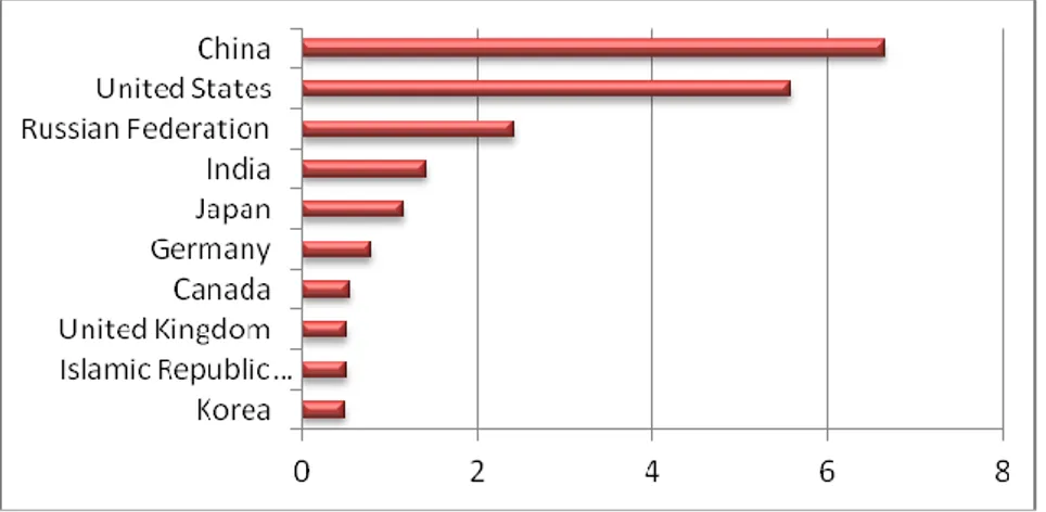
The emissions hovering at higher levels in the colder climates increase in direct proportion with the income and population. As CO2 emissions are closely related to economic growth due to the use of energy, a powerful relationship is observed between per capita income and per capita emission related to energy (World Bank, 2009:13). As SO2 and NOx have direct effect on health and the area they pollute is relatively restricted, although the countries seem quite desirous to reduce these gases, they act reluctantly for reduction of CO2 emissions, especially in the rapid growth periods (Iwata et.al. 2010). Up to the recent time, most anthropogenic greenhouse gases have been emitted by the industrialized countries. However, the share of the developing countries has also increased rapidly and it is expected to increase in future as well. In 2008, two thirds of the world emissions has been caused by 10 countries alone and, among these countries, share of China and USA is above that of all other countries (see Figure 1). These two countries alone have produced 12.1 Gt CO2, which corresponds to about 41% of total CO2 emissions worldwide (IEA; 2010).
Figure 1. Top ten countries with highest carbon emissions in 2008
Many scientists put forward that the increase in the carbon dioxide emissions is one of the most important reasons in the emergence of greenhouse gases, which trigger the global warming and climatic instability (IPCC, 1996; Kaygusuz, 2009). As a result of the threat posed by the global warming on the world ecosystem, a group of developed countries came together and formed the Kyoto Protocol (Halıcıoğlu, 2009). Climate Change Framework Convention and Kyoto Protocol are the most comprehensive multinational effort both in political and geographical sense, being complementary to the national policies and measures to reduce climate change. According to the Protocol, which was entered into force in February 2005, the industrialized countries (as a group) committed to reduce their national emissions in the first commitment period of 2008-2012 by about 5%
compared to the year 1990. Furthermore, while Canada, France, Germany, Italy, Japan, Russian Federation, the UK and the United States have alleviated the climate change; they started G8 Gleneagles Action Plan in July 2005 in order to encourage sustainable development. Signing of Kyoto Protocol, followed with the negotiations about the future of the process as specified by the Protocol, has caused heated discussions on the relationship between carbon dioxide emissions and the economic growth.
In this study, we examined the relationships among CO2 emissions, economic growth and energy consumption. Unlike previous studies, other factors such as nuclear energy generation, foreign trade and urbanization rate that may affect CO2 emission have also been considered. The short term and long-term relationships and causality between CO2 emission, economic growth and energy consumption are analyzed in a multivariate model.
I. LITERATURE REVIEW
The studies in the literature concentrating on the relationship between the economic growth and environmental pollutants (e.g. CO2, SO2 and NOx, etc.) are essentially elaborated in three aspects (Zhang and Cheng, 2009). The first aspect concentrates on the relationship between the environmental pollutants and economic growth. This relationship is closely related to the hypothesis of Environmental Kuznets Curve (“EKC”), which indicates the relationship of the environmental degradation and income increase in a reverse-U form. This hypothesis puts forward that the environmental degradation would increase together with the per capita income in the first stage of the economic growth and then, after reaching to a certain threshold, it would reduce together with the increase in the per capita income. After the first empirical study conducted by Grossmann and Krueger in 1991, a great number of studies have been made to test the relationship between the economic growth and environmental pollutants.
The second aspect of the literature studies concerns relationship of the energy consumption and output. This relationship claims that as the economic growth is closely related to the energy consumption, the economic growth and output may be determined together (Halıcıoğlu, 2009). Kraft and Kraft (1978) used the annual data for the USA for the period of 1947-1974 and found a unidirectional causality from national income to energy consumption. Following this study of Kraft and Kraft (1978), many empirical studies were made on the relationship of the economic growth and energy consumption. The earlier studies used rather a bivariate model and later ones used a multivariate model. However, neither bivariate model nor multivariate model has come to a common result applicable for both of them. For example, findings of Akarca and Long (1980), Yu and Hwang (1984) and Yu and Jin (1992) do not match up with those of Kraft and Kraft (1978). Akarca and Long (1980) have used those data which have been used
by Kraft and Kraft (1978) and tested the relationship of economic growth-energy consumption for the USA for the period of 1947-1974 and found no relationship among those variables. Yu and Hwang (1984) investigated the relationship of the economic growth and energy consumption in the USA for the period of 1947-1979 by using Sims’ causality test and found no causality between two variables. Similarly, Yu and Jin (1992) have not found any relationship between the energy consumption and income in the long run.
Erol and Yu (1987) studied the causality relationship between energy consumption and GDP for the United Kingdom, France, Germany, Italy, Canada and Japan for the period of 1952-1982. They found birectional causality for Japan, unidirectional causality for Canada from energy consumption to GDP and unidirectional causality for Germany and Italy from GDP to energy consumption. No causality relationship has been found for France and the United Kingdom. Stern (1993; 2000) investigated the role of the energy in the development of the US economy in a multivariate model and found out that, when the use of energy is taken as an indicator set against the use of energy, the use of energy causes the economic growth. Soytaş and Sarı (2003) examined the causality between the energy consumption and GDP in the G7 countries, including the United Kingdom and the USA, and in the developing markets, for the period of 1950-1992 and found out that energy consumption has contributed to the economic growth in France, Germany, Japan, Argentine and Turkey.
Third aspect of these studies has appeared upon the combination of two methods above, which study applicability of the relationships. In this approach, all dynamic relations among economic growth, environmental pollutants and energy consumption are studied. (Öztürk and Acaravcı; 2010). Moomaw and Unruh (1997) studied the relationship between CO2, emissions and income level in the developed countries for the period of 1950-1992. There is a trend in form of reverse-U in most of these countries and, furthermore, their threshold values have occurred between 1970-1980. Similarly, Liu (2005), using panel data analysis, made a study on 24 OECD-member countries and used variables such as economic growth, energy consumption and carbon dioxide emissions, concluding that there is EKC based on the carbon dioxide emissions.
Dinda and Coondoo (2006) tested causality relationship between income and emission by using data on 88 countries for the period of 1960-1990, and they concluded that there is a bidirectional causality between two variables. Richmond and Kaufman (2006) studied applicability of EKC for CO2 with respect to the countries that are member or not of OECD, taking into consideration the nuclear energy generation as well. According to the result of the study, although limited in the OECD-member countries, while there is a significant relationship between EKC and CO2, no such relationship is mentioned for the countries, which are not members of OECD. Soytaş et.al. (2007) studied the relationship among the energy consumption, output and carbon emissions in a multivariate model, including the
variables of gross fixed capital and labor in the USA for the period of 1960-2004. While no causality was found either between income and carbon emissions or between energy consumption and income, the energy consumption is granger cause of the carbon emissions in the long run. Using cointegration and error correction models, Ang (2007) investigated the long term relationship among the carbon dioxide emissions, energy consumption and output in France for the period of 1960-2007. Ang (2008) examined the relationship among output, CO2 emissions and energy consumption by using the error correction model in Malaysia for the period of 1971-1998. The results verify existence of a relationship in the long term among the variables and CO2 emissions and energy consumption has a positive relationship with the output in the long term. Both in long and short term, there is a powerful causality from energy consumption to economic growth. Apergis and Payne (2009) examined the relationships CO2 emissions, energy consumption and output in 6 Central American countries for the period of 1971-2004. They found a unidirectional causality from energy consumption to output and bidirectional one between the energy consumption and real output in the long term and bidirectional causality between the energy consumption and emissions in the long term. Soytaş and Sarı (2009) investigated the relationship among income, carbon emissions and energy consumption for Turkey and found no causality between income and emissions, but a unidirectional causality from carbon emissions to energy consumption. Contrary to Soytaş and Sarı (2009), Halıcıoğlu (2009) concluded that there is a bidirectional causality between carbon emissions and economic growth both in long and short term in Turkey. Zhang and Cheng (2009), using data in the period of 1960-2007 for China, studied causality among energy consumption, carbon emissions and economic growth and estimated that there is a unidirectional Granger causality from economic growth to energy consumption, and in case of energy consumption, to the emissions in the long term. Jalil and Mahmud (2009) examined the long-term relationship among carbon emissions, energy consumption, income and foreign trade in the period of 1970-2005 for China. They found that EKC was applicable and that the carbon emissions were determined in long term depending on income and energy consumption. Causality test results indicate that there is a unidirectional causality from economic growth to CO2 emissions.
Ghosh (2010) investigated the relationship between carbon emissions and economic growth for India over the period 1971-1976 and found no relationship between two variables in the long term, but concluded that there is a bidirectional causality in the short period. Hatzigeorgiou et.al. (2011) examined the causality among CO2 emissions, GDP and energy density for Greece. They found a unidirectional causality between GDP and energy density and GDP and CO2 from GDP to energy density and from GDP to CO2 emissions. And there is a bidirectional causality between CO2 and energy density. Menyah and Woldo-Rufael (2010) tested the long-term relationship among economic growth, pollutant emissions and energy consumption in the case of South Africa by employing time
series data of 1965-2006. They found a unidirectional causality operating from the pollutant emissions to economic growth, from energy consumption to economic growth and from energy consumption to CO2 emissions. Apergis and Payne (2010) investigated the causality relations among carbon dioxide emissions, energy consumption and growth in the Commonwealth of Independent States for the 1992-2004 period. In the short term, both energy consumption and economic growth are Granger cause of the carbon dioxide emissions. In the long term, there is a bidirectional causality between the carbon dioxide emissions and energy consumption. Lean and Smyth (2010) studied the causality relationship among CO2 emissions, power consumption and output for ASEAN during the period 1980-2006. The empirical results show a unidirectional causality in the long term from power consumption and emissions to economic growth. Taking account of the role of the nuclear energy, Iwata et.al. (2010) estimated existence of EKC for France over the period 1960-2003. The findings show that the EKC is applicable for France. Furthermore, there is a unidirectional running from other variables, including nuclear energy to CO2. The finding of the unidirectional causality from nuclear energy to CO2 shows that the nuclear energy plays a significant role in reducing CO2 emissions. Narayan and Narayan (2010) investigated the existence of the EKC, basing on the short-term and the long-term income flexibility of 43 developing countries. Finally, the income flexibility was found to be lower in the long term than the short term only for the Middle Eastern and South Asian countries. This result indicates that the carbon dioxide emissions in the countries mentioned before have reduced together with increase in the income.
Pao and Tsai (2011) tested the causality among CO2 emissions, energy consumption, FDI and economic growth in the BRIC countries (Brazil, Russian Federation, India and China) in a multivariate model. They found a bidirectional causality between output-emission and output-energy consumption and a unidirectional causality from energy consumption to emissions. They have reached to results supporting EKC hypothesis. Lotfalipour et.al. (2011) have, using Toda-Yamamoto causality tests, tested causality relationship among economic growth, CO2 emissions and fossil fuels in Iran. They found a unidirectional causality from GDP and energy consumption to CO2 emissions. Wang et.al. (2011) examined the causality among CO2 emissions, energy consumption and economic growth in China for the 1995-2007 period. And they found a bidirectional causality among CO2 emissions, energy consumption and economic growth in China. Hossain (2011) investigated the causality relations among CO2 emissions, energy consumption, economic growth, trade gap and urbanization in the newly industrializing countries. While, according to the causality test results, there is no causality among those variables in the long term in these countries, there is a unidirectional causality in the short term running from economic growth and trade gap to CO2 emissions, from economic growth to energy consumption, from trade gap to economic growth, from urbanization to economic growth and from trade to urbanization.
II. DATA
The study covers the period of 1960-2004 and annual data were used. All data were taken from the World Development Indicators CD-ROM (2007). CO2, GDP, EN, NUC, TR and URB, respectively, show emissions measured in metric ton per capita, real GDP per capita income, energy consumption measured as oil equivalent per capita, ratio of the power generated from nuclear resource to the total power generation, ratio of sum of import and export in GDP and ratio of urban population to total population. The logarithms of all series were taken.
III. METHODOLOGY A. UNIT ROOT
In the econometric estimations, stationary of time series is important. It
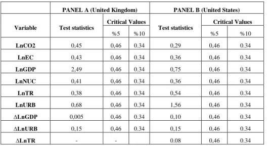
has been shown that working with Granger and Newbold (1974) nonstationary series may lead to false regression problem. For this reason, firstly, the stationarity properties of the data using unit root test, also called KPSS test, developed by Kwiatkowski, Phillips, Schmidt and Shin (1992) is investigated. Table 1 shows results of unit root test.
Table 1. KPSS Unit Root Test
PANEL A (United Kingdom) PANEL B (United States)
Variable Test statistics
Critical Values Test statistics Critical Values %5 %10 %5 %10 LnCO2 0,45 0,46 0.34 0,29 0,46 0.34 LnEC 0,43 0,46 0.34 0,36 0,46 0.34 LnGDP 2,49 0,46 0.34 0,75 0,46 0.34 LnNUC 0,41 0,46 0.34 0,36 0,46 0.34 LnTR 0,38 0,46 0.34 0,54 0,46 0.34 LnURB 0,68 0,46 0.34 1,56 0,46 0.34 ∆LnGDP 0,005 0,46 0.34 0,10 0,46 0.34 ∆LnURB 0,15 0,46 0.34 0,15 0,46 0.34 ∆LnTR - - 0.08 0,46 0.34
Optimal lag in the KPSS test selected by Schwartz Information Criterion (SIC). ∆ shows the first difference operator, ln stands for logarithm.
In Table 1, Panel A shows the results of KPSS unit root test for the United Kingdom and Panel B for the USA. As it may be seen from the table, null hypothesis which states that all series are stationary in level, except for GDP and URB series in Panel A and GFDP, URB and TR series in Panel B, cannot be rejected in the significance level of 5%. In contrast, when the nonstationary series
are differenced, null hypothesis that stationary cannot be rejected at the significance level of 5% for all data series. In summary, KPSS test results show that the variables are not integrated in the same level.
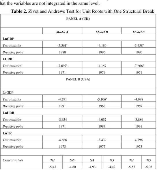
Table 2. Zivot and Andrews Test for Unit Roots with One Structural Break PANEL A (UK)
Model A Model B Model C
LnGDP Test statistics -5.561a -4.180 -5.458b Breaking point 1980 1996 1980 LURB Test statistics -7.697a -4.157 -7.606a Breaking point 1971 1979 1971 PANEL B (USA) LnGDP Test statistics -4.791 -5.106a -4.998 Breaking point 1991 1968 1969 LnURB Test statistics -3.654 -4.052 -3.889 Breaking point 1971 1987 1991 LnTR Test statistics -4.666 -3.439 4.796 Breaking point 1973 1977 1973 Critical values %1 %5 %1 %5 %1 %5 -5,43 -4,80 -4,93 -4,42 -5,57 -5,08
Critical values indicate values taken from Zivot and Andrews (1992). a
Significant at 1%b Significant at 5%
Many authors have indicated that conventional unit root tests are not relevant for variables that are with inclusion of structural changes. Zivot and Andrews (1992) introduce methods to endogenously search for breakpoint and test for the presence of a unit root when the time series process has a breaking trend. The Zivot-Andrews (henceforth, ZA) tests are represented by following regression equations:
ModelA: ) 1 ( 1 3 2 1 1 0 t j t A k j j t A A t A A t d t DU d d
ModelB: ) 2 ( 1 3 2 1 1 0 t j t B k j j t B B t B B t d t DT d d
ModelC: ) 3 ( 1 4 3 2 1 1 0 t j t C k j j t C t C C t C C t d t DU DT d d
t TB if DUt =1 and 0 otherwise; and DTt=t-TB and 0 otherwise. Here TB denotes the break point. Model A allows for break in the intercept. Model B allows for a break in the trend function. Model C combines the constant and the break in the trend functions slope, in other words reflects both effects (constant and slope).
We report the results from Zivot and Andrews (1992) one endogenous break test in Table 2. Breaking years indicate differences depending on the different models. In Table 2, Panel A shows ZA unit root test results for the United Kingdom. There is a structural break in GDP series in 1980 according to Model A and Model C and in 1996 according to Model B. As the absolute value of the test statistic is higher than the critical value in Model A and Model C, the null hypothesis for GDP is rejected in the significance level of 5%. In Model B, the test statistic is smaller than the critical value and the unit root the null hypothesis cannot be rejected. There is a structural break in URB series in 1971 according to Model A and Model C and in 1979 according to Model B. Likewise, while the unit root hypothesis is rejected according to Model A and Model C, the null cannot be rejected according to Model B. In other words, when the breaks are taken into consideration, for both variables, the null hypothesis of a unit root cannot be rejected at their levels according to Model A and Model C. However, according to Model B, the null hypotheses are the series has unit root can be rejected for both variables.
Panel B contains the results of the ZA unit root test for GDP, URB and TR series for USA. For GDP series, Model A shows that there is a structural break in 1991, Model B in 1968 and Model C in 1969. For URB and TR series, respectively, Model A indicates that there are structural break in 1971 and 1973, Model B in 1987 and 1977 and Model C in 1991 and 1973. For three series all, as the absolute value of the test statistic is smaller than the critical value in Model C and Model A, the unit root hypothesis cannot be rejected in the significance level of %5. The results show that the series are not integrated in the same level, verifying those results, which have been found with KPSS test previously1.
B. COINTEGRATION
Secondly, it has been investigated whether there is a long-term relation among the series. In the study, the cointegration method developed by Pesaran et.al. (2001) and Banerjee et.al. (1998), was preferred. The reason is that both methods can be applied independently whether the regressors are I(0) or I(1) and avoids the pre-test with standard cointegration analysis. Furthermore, unlike other conventional cointegration tests, the bound test can be applied to the studies that have a small sample size (Narayan, 2005). And as to this study, both the number of observation is limited (n=44), and the series are not integrated in the same level in presence of the structural breaks.
For application of the bound test, first the unrestricted error correction model (UECM) is estimated. For this reason, the following error correction model was estimated in order to estimate the long-term relation among the variables. .
) 4 ( ln ln ln ln ln 2 ln ln ln ln ln ln 2 ln 2 ln 1 1 13 1 12 1 11 1 10 1 9 1 8 1 7 1 6 1 5 1 4 1 3 1 2 1 0
t t t t t t i t n i i i t n i i i t n i i i t n i i i t n i i i t n i i URB TR NUC GDP EC CO URB TR NUC GDP EC CO t a COIn the ARDL approach, test for cointegration is carried out by testing of the null hypothesis of no cointegration (H0:a8 a9 a10a11a12a130) against the alternative using the F-test critical values tabulated by Pesaran et.al. (2001). According to Pesaran et.al. (2001), if the calculated F statistic falls below the lower critical value, the null hypothesis is not rejected, indicating no cointegration. If the calculated F statistic exceeds the upper critical value, the null hypothesis is rejected. If, however, the calculated F statistic falls within the lower and upper critical values, result is inconclusive. However, according to Narayan (2005), the critical values calculated and reported by Pesaran et.al. (2001) are generated sample size 500, 1000, 20000 and 40000 replications respectively. Because these critical values are based on large samples, they are not usable for small sample size. For this reason, Narayan (2005) calculated new critical values for sample sizes ranging from 30-80 observations (Narayan, 2005:1981). In the approach of Banerjee et.al.(1998), test for cointegration is carried out by testing statistical significance of
8 coefficient in the equation (4). The calculated t-statistic is compared to the t-test critical values tabulated by Pesaran et.al. (2001) If calculated t statistics falls above the upper bound, it implies cointegration.One of the more important issues in applying ARDL is choosing the order of the distributed lag function. Since all observations are annual and the number of observations is limited, as the maximum lag length in the ARDL model is set 3. The optimal number of lags is selected based on Schwarz Information Criterion (SIC) and the absence of residual serial correlation has also confirmed the correct order of lag selection.
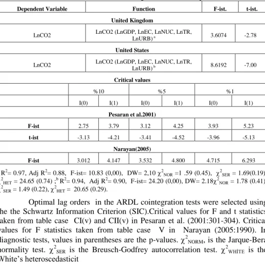
Table 3. Bounds Test Results for Long-Run Relationship
Dependent Variable Function F-ist. t-ist.
United Kingdom
LnCO2 LnCO2 (LnGDP, LnEC, LnNUC, LnTR,
LnURB) a 3.6074 -2.78 United States
LnCO2 LnCO2 (LnGDP, LnEC, LnNUC, LnTR,
LnURB) b 8.6192 -7.00 Critical values
%10 %5 %1
I(0) I(1) I(0) I(1) I(0) I(1)
Pesaran et al.2001) F-ist 2.75 3.79 3.12 4.25 3.93 5.23 t-ist -3.13 -4.21 -3.41 -4.52 -3.96 -5.13 Narayan(2005) F-ist 3.012 4.147 3.532 4.800 4.715 6.293 a
R2= 0.97, Adj R2= 0.88, F-ist= 10.83 (0,00), DW= 2,10 2NOR =1 .59 (0.45), 2
SER = 1.69(0.19), 2
HET = 24.65 (0.74) ;b R2= 0.94, Adj R2= 0.90, F-ist= 24.20 (0,00), DW= 2.182NOR = 1.78 (0.41), 2
SER = 1.49 (0.22), 2
HET = 20.65 (0.29).
Optimal lag orders in the ARDL cointegration tests were selected using the the Schwartz Information Criterion (SIC).Critical values for F and t statistics taken from table case CI(v) and CII(v) in Pesaran et al. (2001:301-304). Critical values for F statistics taken from table case V in Narayan (2005:1990). In diagnostic tests, values in parentheses are the p-values. 2NORM, is the Jarque-Bera normality test. 2SER is the Breusch-Godfrey autocorrelation test.
2
WHİTE is the White’s heteroscedasticit
In Table 3, Panel A and Panel B show the results of the cointegration test estimated by the model (4). As it may be seen from the Panel B, the F-statistic testing the long-term relationship for the USA is 8.61, the t-statistic is -7,00; both of them exceed the upper critical values taken from Narayan (2005) and Pesaran et al. (2001). According to the cointegration test results in Panel B, the null of no cointegration among the variables is rejected in the significance level of 1%. The cointegration test results of the model estimated for the United Kingdom are given in panel A. As the value of the F statistic testing the long-term relationship falls inside the lower and upper critical values taken from Narayan (2005) and Pesaran et.al. (2001), no decision can be made. However, the bound test allows testing the cointegration even in case when no decision can be given on cointegration. In such case, the most effective way to verify the cointegration is the application of ECM version of ARDL model (Bahmani-Oskooe and Nasir, 2004). Furthermore, the
diagnostic tests of the models have been given under the table and both models passes through all diagnostic tests.
C. LONG RUN AND ECM
Once, the long-run relationship is identified, then, second stage of the ARDL approach is to estimate the coefficient of long-run cointegrating relationship. Long-run cointegrating regression is specified as follows:
) 5 ( ln ln ln ln ln 2 ln 2 ln 0 7 0 6 0 5 0 4 0 3 1 2 1 0 t i t n i i i t n i i i t n i i i t n i i i t n i i i t n i i URB a TR a NUC a GDP a EC a CO a t a a CO
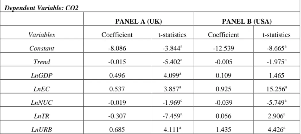
The results of the model 5 estimated for the USA and the United Kingdom are given in Table 4. While the effect of GDP on CO2 is positive and statistically significant in the United Kingdom, it is positive, but statistically insignificant, in the USA. In other words, while the economic growth in the United Kingdom has a significant effect on CO2, it has no effect in the USA. An increase of 1% in the economic growth in the United Kingdom causes an increase of 0.4% in CO2. Long-term effect of the energy consumption in both countries is positive and statistically significant. Increase in the energy consumption causes an increase in CO2 in both countries in the long term. The long-term elasticity of the energy consumption with respect to CO2 is higher in USA (0.9) than the United Kingdom (0.5). Effect of foreign trade on CO2 in the USA is positive and its effect in the United Kingdom is negative and statistically significant. The coefficient of the nuclear energy is negative and statistically significant for both countries. In the long term, an increase in the nuclear energy generation causes reduction in CO2 in both countries. And the urbanization rate is statistically significant and has a positive effect in both countries.
Table 4. Estimated Long-Run Coefficients Dependent Variable: CO2
PANEL A (UK) PANEL B (USA)
Variables Coefficient t-statistics Coefficient t-statistics
Constant -8.086 -3.844a -12.539 -8.665a Trend -0.015 -5.402a -0.005 -1.975c LnGDP 0.496 4.099a 0.109 1.465 LnEC 0.537 3.857a 0.925 15.256a LnNUC -0.019 -1.969c -0.039 -5.749a LnTR -0.307 -7.459a 0.056 2.906a LnURB 0.685 4.111a 1.435 4.426a
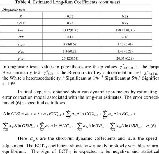
Table 4. Estimated Long-Run Coefficients (continues) Diagnostic tests R2 0.97 0.98 Adj R2 0.94 0.98 F-ist 30.12(0.00) 128.43 (0,00) DW 2.14 2.18 2NOR 0.79(0.67) 1.78 (0.41) 2SER 1.46(0.22) 1.49 (0.22) 2 HET 23.12(0.51) 20.65 (0.29)
In diagnostic tests, values in parentheses are the p-values. 2NORM, is the Jarque-Bera normality test. 2SER is the Breusch-Godfrey autocorrelation test.
2
WHİTE is the White’s heteroscedasticity. a
Significant at 1% b Significant at 5%.c Significant at 10%
In final step, it is obtained short-run dynamic parameters by estimating an error correction model associated with the long-run estimates. The error correction model (6) is specified as follows
) 6 ( ln ln ln ln ln 2 ln 2 ln 0 8 0 7 0 6 0 5 0 4 1 3 1 2 1 0 t i t n i i i t n i i i t n i i i t n i i i t n i i i t n i i t URB a TR a NUC a GDP a EC a CO a ECT t a a CO
Here ajis are the short-run dynamic coffecients and
a
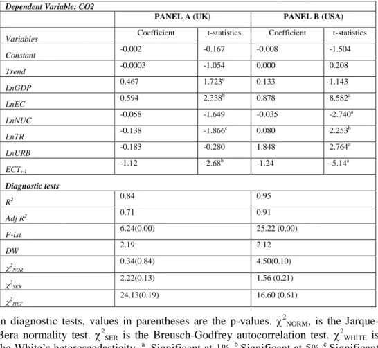
2is the speed of adjustment. The ECTt-1 coefficient shows how quickly or slowly variables return to equilibrium. The sign of ECTt-1 is expected to be negative and statistically significant.Table 5 shows the estimation results of the model for the short term. In the model, the error correction term (ECTt-1) is estimated as -1.12 in Panel A and -1.24 in Panel B. In both panels, the sign of the ECTt-1 is, as expected, negative and statistically significant at the 5% level. Estimated coefficient of ECTt-1 is greater than 1, suggesting that as stated by Narayan and Smyth (2006) the system shall reach to the long-term equilibrium after fluctuation. This fluctuation shall decrease each time, ensuring return to equilibrium in the long term. Furthermore, according to Banerjee et.al. (1998), the statistical significance of the error correction term is high and it is the further evidence of co integration between among the variables. In our model as well, the lagged error correction term is statistically significant at the %5 level, verifying presence of a long-term relationship among the variables in both countries.
Table 5. Estimated Short-Run Error Correction Model (ECM) Dependent Variable: CO2
PANEL A (UK) PANEL B (USA)
Variables Coefficient t-statistics Coefficient t-statistics
Constant -0.002 -0.167 -0.008 -1.504 Trend -0.0003 -1.054 0,000 0.208 LnGDP 0.467 1.723 c 0.133 1.143 LnEC 0.594 2.338 b 0.878 8.582a LnNUC -0.058 -1.649 -0.035 -2.740 a LnTR -0.138 -1.866 c 0.080 2.253b LnURB -0.183 -0.280 1.848 2.764 a ECTt-1 -1.12 -2.68 b -1.24 -5.14a Diagnostic tests R2 0.84 0.95 Adj R2 0.71 0.91 F-ist 6.24(0.00) 25.22 (0,00) DW 2.19 2.12 2NOR 0.34(0.84) 4.50(0.10) 2SER 2.22(0.13) 1.56 (0.21) 2HET 24.13(0.19) 16.60 (0.61)
In diagnostic tests, values in parentheses are the p-values. 2NORM, is the Jarque-Bera normality test. 2SER is the Breusch-Godfrey autocorrelation test.
2
WHİTE is the White’s heteroscedasticity. a
Significant at 1% b Significant at 5%.c Significant at 10%.
As it may be seen from Panel A in Table 5, in the United Kingdom the economic growth has a weak positive effect on CO2 in the short term. The coefficient of GDP is statistically significant at the 10% level. The energy consumption has positive effect on CO2 in the short term and the coefficient of the energy consumption is statistically significant at the level of 5%. An increase of 10% in the energy consumption causes an increase of about 6 percent in CO2. Furthermore, the elasticity of the energy consumption with respect to CO2 is higher in the short term than the long term. The coefficient of the foreign trade is negative and significant at the 10% level. In the short term, the foreign trade has weak negative effect on CO2. Unlike the long term, the nuclear energy generation and urbanization rate have no effect on CO2 in the short term.
Panel B part of the Table 5 shows the short-term effects for the USA. While, as it is in the long term, GNP has no effect on CO2 in the short term, energy consumption, foreign trade and urbanization rate have a significant and positive
effect on CO2. Short-term elasticity of the energy consumption with respect to CO2 is, contrary to the United Kingdom, smaller in the long term than the short term. An increase of 10% in the energy consumption causes an increase of 8.7% in CO2 in the short term. Effect of the nuclear energy on CO2 is also significant and negative in the short term, as it is in the long term. Long and short term elasticity of the nuclear energy with respect to CO2 are quite close to each other.
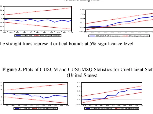
As shown in the bottom of Tables, both models (5) and (6) pass all diagnostic tests. These tests show that there is no evidence of autocorrelation and that the models pass tests for normality and those proving that the error is normally distributed. In order to test the structural stability of the estimated models, the cumulative sum (CUSUM) and cumulative sum of squares (CUSUMSQ) test have also been performed. Figure 2 and 3 indicate a graphical presentation of these two tests. It can be seen from the figures that the plot of CUSUM stay within the critical 5% bound for all equations and CUSUMQ statistics does not exceed the critical boundaries that confirms the long-run relationships between variables and also shows stability in the coefficient over the sample period.
Figure 2. Plots of CUSUM and CUSUMSQ Statistics for Coefficient Stability
(United Kingdom)
The straight lines represent critical bounds at 5% significance level
Figure 3. Plots of CUSUM and CUSUMSQ Statistics for Coefficient Stability
(United States)
The straight lines represent critical bounds at 5% significance level
D. CAUSALITY
To estimate the causal relationship among variables, Toda and Yamamoto (1995) test for long causality is utilized. The main advantage of Toda-Yamamoto procedure is that it can be applied independently whether the regressors are I(0) or
-15 -10 -5 0 5 10 15 84 86 88 90 92 94 96 98 00 02 04 CUSUM 5% Significance -0.4 0.0 0.4 0.8 1.2 1.6 84 86 88 90 92 94 96 98 00 02 04 CUSUM of Squares 5% Significance
-15 -10 -5 0 5 10 15 84 86 88 90 92 94 96 98 00 02 04 CUSUM 5% Significance -0.4 0.0 0.4 0.8 1.2 1.6 84 86 88 90 92 94 96 98 00 02 04 CUSUM of Squares 5% Significance
I(1) or whether regressors are coinegrated (Toda and Yamamoto: 1995:227). In order to test causality among the variables, following system equation have been estimated. (7)
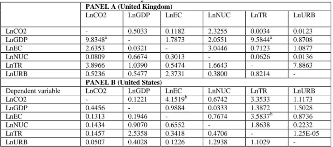
Table 6 shows Toda and Yamamoto causality results. As it may be seen from Panel B, there is no causality between energy consumption and economic growth in the USA, neither from growth to energy consumption nor from energy consumption to growth. Absence of any causality between two variables supports the neutrality hypothesis putting forward that energy consumption has no effect on economic growth. Furthermore, this finding coincide findings of Yu and Hwang (1984), Yu and Choi (1985), Yu et.al. (1988), Chang (1996), Murray and Nan (1996), Soytaş and Sarı (2003), Chontanawat et.al. (2006), Soytaş et.al. (2007), Narayan and Prasad (2008) that had previously found that there is no causality for the USA. And there is no causality between CO2 and economic growth, neither from growth to CO2 nor from CO2 to growth. There is a unidirectional Granger causality between energy consumption and CO2 and foreign trade, running from energy consumption to CO2 and from foreign trade to energy consumption.
Table 6. Toda-Yamamoto Causality Test
PANEL A (United Kingdom)
LnCO2 LnGDP LnEC LnNUC LnTR LnURB
LnCO2 - 0.5033 0.1182 2.3255 0.0034 0.0123 LnGDP 9.8348a - 1.7873 2.0551 9.5844a 0.8708 LnEC 2.6353 0.0321 - 3.0446 0.7123 1.0877 LnNUC 0.0809 0.6674 0.3013 - 0.0626 0.0136 LnTR 3.8966 1.0390 0.5474 1.6643 - 7.8863 LnURB 0.5236 0.5477 2.3731 0.3800 0.8214 -
PANEL B (United States)
Dependent variable LnCO2 LnGDP LnEC LnNUC LnTR LnURB
LnCO2 - 0.1221 4.1519b 0.6742 3.3533 1.1173 LnGDP 0.4456 - 0.9884 0.0333 1.3872 1.5028 LnEC 0.1313 0.1946 - 0.7674 3.5837b 0.8736 LnNUC 0.1434 0.9070 0.6552 - 1.8638 0.2232 LnTR 0.1457 2.5358 0.3418 0.4706 - 1.25E-05 LnURB 0.0507 0.4028 0.1226 1.2938 1.1029 - a Significant at 1% b Significant at 5%.
Table 6 Panel A shows the results of Toda and Yamamoto causality test for the United Kingdom. While there is no causality in any direction between CO2 and energy consumption, there is also no causality relationship between economic growth and energy consumption. This finding demonstrates that the neutrality hypothesis is applicable for the United Kingdom and coincides with findings of Erol and Yu (1987), Soytaş and Sarı (2003), Lee (2006), Chontanawat et.al.(2006)
for the United Kingdom. There is a unidirectional causality between GDP and CO2 and foreign trade. The null hypothesis that CO2 is not Granger cause of the economic growth as well as the null hypothesis that foreign trade is not Granger cause of growth is rejected. A unidirectional causality from CO2 to GDP shows that a reduction in CO2 would cause reduction in growth and, consequently, the policies for reduction of CO2 may require sacrifice from growth.
CONCLUSION
In this study, the relations among carbon emissions, the economic growth and energy consumption in a multivariate model, which includes nuclear energy generation, foreign trade and urbanization variables, is investigated in the case of the United Kingdom and the USA by employing data of 1960-2004. Unit root test results show that the variables are not integrated in the same level. And the unit root tests with structural break support the results of unit root test found by KPSS. Cointegration test results show that when CO2 is considered as a dependent variable, there is a long-term relationship among the variables in question.
Energy consumption, foreign trade and urbanization have significant and positive effect on the carbon dioxide emissions and the electric generated from nuclear energy has negative effect for in the short term for the USA. In the long term, the energy consumption, foreign trade and urbanization ratio have significant and positive effect on the carbon dioxide emissions. And while the economic growth has no effect on the carbon dioxide emissions, the power generated from the nuclear energy has a significant and negative effect on the carbon dioxide emissions. For the United Kingdom, in the short term, the economic growth, energy consumption and foreign trade have significant and positive effect on the carbon dioxide emissions. In the long term, the economic growth, energy consumption and urbanization ratio have a significant and positive effect on the carbon dioxide emissions.
The foreign trade and power generated from the nuclear energy have negative and significant effect on the carbon dioxide emissions. And thus the importance of the role played by the nuclear energy in reducing carbon dioxide emissions in the long term has been empirically proved for both countries. Economic growth has not effect carbon dioxide emissions in the short term in the USA. Power generated from the nuclear energy and urbanization in the United Kingdom have no effect on the carbon dioxide emissions in the short term.
While the long-term elasticity of the energy consumption with respect to carbon dioxide emissions is (0.537) in the United Kingdom and (0.925) in the USA, the short term elasticity is (0.594) in the United Kingdom and 0.878 in the USA. According to this elasticity values, long-term elasticity (0.537) of the energy consumption with respect to carbon dioxide emissions in the United Kingdom is below those of the short term (0.594). In the USA, the long-term elasticity value
(0.925) is higher than the short-term elasticity value (0.878). According to these data, depending on the energy consumption over time, it may be said that the environmental quality in the USA is not better compared to the United Kingdom. This situation shows that any increase occurring in the energy consumption in a certain period would cause more carbon dioxide emission and thus the environment shall be polluted more.
According to Granger causality test results, there is no causality between energy consumption and economic growth in the USA, neither from growth to energy consumption nor from energy consumption to growth. While there is a unidirectional causality from energy consumption to CO2 between the carbon dioxide emissions and energy consumption, there is no causality relationship between the emissions and economic growth. There is no causality relationship among other variables. There is unidirectional causality from energy consumption to CO2 and that there is no causality between energy consumption and economic growth indicates that it is easy and possible to establish and implement energy policies in this country to reduce environmental pollution without slowing down the economic growth.
While there is no causality between the carbon dioxide emissions and energy consumption in the United Kingdom, there is no causality between the economic growth and energy consumption as well. This finding indicates that economic growth objectives and energy policy goals may be easily implemented easily. And there is unidirectional causality among the economic growth and carbon emissions and foreign trade, running from carbon emissions to economic growth and from foreign trade to economic growth. That the reduction in CO2 causes a reduction in the growth shows that it is not possible to reduce emissions without any sacrifice from the growth in this country.
On the other hand, there is a significant and negative effect of the power generated from the nuclear energy on the carbon dioxide emissions both in the USA and the United Kingdom. This finding show that while the carbon dioxide emissions increase together with the economic growth, any attempt for reduction of the emissions do not affect the economic development. However, it should be taken into consideration that high amount of administration costs is required for security in order to protect environment and human health against any potential accident that may occur during generation of nuclear energy. For this reason, when taking a decision on the matter of nuclear energy, we should also consider potential threats in addition to the advantages of the nuclear energy in reducing the carbon dioxide emissions. Furthermore, it is useful to utilize alternative energy resources such as solar energy to reduce carbon emissions. It would both reduce dependence on nuclear energy and be effective in diversification of the risks that may arise due to use of nuclear energy.
Estimation about relationship between the economic growth, CO2 and energy consumption and effect of the nuclear energy on CO2 in both countries
show that these countries have a wide area of action to establish their respective energy policies towards alternative and renewable energy resources in an environmental-friendly and sustainable manner. Both countries may diversify their energy policies in this direction and thus minimize environmental pollution and increase the energy supply constantly and assuredly in the long term. Furthermore, taking into consideration their economic volume, both countries may act as leaders in leaving a cleaner and livable environment to the future generations by giving assistance for development and widespread use of alternative and renewable energy technologies.
REFERENCES
AKARCA, Ali; LONG, Thomas Veach (1980), “On the Relationship Between Energy And GNP: A Reexamination”, Journal of Energy And Development, 5; 326– 331.
ANG, James B. (2007), “CO2 Emissions, Energy Consumption, And Output in France”, Energy Policy, 35, 4772-4778.
ANG, James B. (2008), “Economic Development, Pollutant Emissions And Energy Consumption In Malaysia”, Journal of Policy Modeling, 30; 271–278.
APERGIS, Nicholas; PAYNE, James E. (2009), “CO2 Emissions, Energyusage, and Output In Central America”, Energy Policy, 37; 3282–3286.
APERGIS, Nicholas; PAYNE, James E. (2010), “The Emissions, Energy Consumption, And Growth Nexus: Evidence From The Commonwealth Of Independent States”, Energy Policy, 38, 650–655.
BAHMANI-OSKOOEE, Mohsen; NASIR, A.B.M. (2004), “ARDL Approach To Test The Productivity Bias Hypothesis”, Review Of Development Economic; 8, 483-488.
BANERJEE, Anindya; DOLADO, Juan; MESTRE, Ricardo (1998), “Error-Correction Mechanism Tests For Cointegration In A Single-Equation Framework”, Journal of Time Series Analysis, 19; 267–283.
CHENG, B.S (1996), “An Investigation Of Cointegration And Causality Between Energy Consumption And Economic Growth”, Journal of Energy and Development, 21; 73–84.
CHONTANAWAT, Jaruvan; HUNT, Lester.C and PIERSE, Richard (2006), “Causality Between Energy Consumption And GDP: Evidence From 30 OECD And 78 non-OECD Countries”. Surrey Energy Economics Discussion Paper Series 113.
DINDA, Soumyananda; COONDOO, Dipankor (2006), “Income And Emission: A Panel Data-Based Cointegration Analysis” Ecological Economics, 57; 167– 181.
ENDERS, Walter (1995), Applied Econometric Time Series, First Ed., Wiley, New York.
EROL, Umit; YU, Eden.S.H (1987), “On The Relationship Between Electricity And Income For Industrialized Countries”, Journal of Electricity and Employment, 13, 113–122.
GHOSH, Sajal (2010), “Examining Carbon Emissions Economic Growth Nexus For India: A Multivariate Cointegration Approach”, Energy Policy, 38; 3008– 3014.
GRANGER, Clive.W.J; NEWBOLD, Paul (1974), “Spurious Regressions In Econometrics”, Journal of Econometrics, 2, 111-120.
GROSSMAN, Gene M. ; KRUEGER, Alan B. (1991), “Environmental Impacts Of A North American Free Trade Agreement. National Bureau Of Economics Research Working Paper”, No.3194, NBER, Cambridge.
HALICIOĞLU, Ferda (2009), “An Econometric Study Of CO2 Emissions, Energy Consumption, Income And Foreign Trade In Turkey”, Energy Policy, 37; 1156-1164.
HATZIGORGIOU, Emmanouil; POLATIDIS, Heracles and HARALAMBOPOULOS, Dias (2011), “CO2 Emissions, GDP And Energy Intensity: A Multivariate Cointegration And Causality Analysis For Greece”, 1977–2007. Applied Energy, 88; 1377–1385.
HOSSAIN, Sharif (2011), “Panel Estimation For CO2 Emissions, Energy Consumption, Economic Growth, Trade Openness And Urbanization Of Newly Industrialized Countries”, Energy Policy, 39; 6991-6999.
INTERNATIONAL ENERGY AGENCY (IEA) (2010), CO2 Emissions From Fuel Combustion (2010 Edition), France.
IWATA, Hiroki; OKADA, Keisuke and SAMRETH, Sovannroeun (2010), “Empirical Study On The Environmental Kuznets Curve For CO2 In France: The Role Of Nuclear Energy”, Energy Policy, 38; 4057-4063.
IPCC. (1996), IPCC Second Assessment On Climate Change. International Panel On Climate Change. Cambridge University Pres, Cambridge, UK.
JALIL, Abdul; MAHMUD, Syed F. (2009), “Environment Kuznets Curve For CO2 Emissions A Cointegration Analysis”, Energy Policy, 37; 5167–5172.
JOHANSEN, Soren (1991), “Estimation And Hypothesis Testing Of Cointegration Vectors in Gaussian Vector Autoregressive Models” Econometrica, 5; 1551– 1580.
KAYGUSUZ, Kamil (2009), “Energy And Environmental Issues Relating To Greenhouse Gas Emissions For Sustainable Development In Turkey”. Renewable And Sustainable Energy Reviews, 13; 253-270.
KRAFT, J; KRAFT, A (1978), “On The Relationship Between Energy And GDP”, Journal of Energy and Development, 3; 401-403.
KWIATKOWSKI, Denis; PETER, C. B. Phillips; PETER, Schmidt, and YONGCHEOL Shin (1992), “Testing The Null Hypothesis Of Stationary Against The Alternative Of A Unit Root”, Journal of Econometrics, 54; 159-178.
LEAN; Hooi-Hooi; SMYTH, Russell (2010), “CO2 Emissions, Electricity Consumption And Output In ASEAN”, Applied Energy, 87; 1858–1864. LEE, Chien-Chiang (2006), “The Causality Relationship Between Energy
Consumption And GDP in G-11 Countries Revisited”, Energy Policy, 34; 1086–1093.
LIU, Xuemei (2005), “Explaining The Relationship Between CO2 Emissions And National Income – The Role Of Energy Consumption”, Economic Letters, 87; 325-328.
LOTFALIPOUR, Mohammed Reza; FALAHI, Mohammed Ali and ASHENA Malihe (2011), “Economic Growth, CO2 Emissions And Fossil Fuels Consumption In Iran”, Energy , 35; 5115-5120.
MENYAH, Kojo; YEMENA; Wolde-Rufael (2010), “Energy Consumption, Pollutant Emissions And Economic Growth In South Africa”, Energy Economics, 32; 1374–1382.
MOOMAW, William.R; UNRUH, Gregory .C (1997), “Are Environmental Kuznets Curves Misleading Us? the Case Of CO2 Emissions”, Environment and Development Economics, 2; 451-463.
MURRAY, D.A; NAN, G.D (1996), “A Definition Of The Gross Domestic Product-Electrification Interrelationship”, Journal of Energy and Development, 19; 275–283.
NARAYAN, Paresh K. (2005), “The Saving And Investment Nexus For China: Evidence From Cointegration Tests”, Applied Economics. 37; 1979-1990. NARAYAN, Paresh. K; PRASAD, Arti (2008), “Electricity Consumption-Real GDP
Causality Nexus: Evidence From A Bootstrapped Causality Test For 30 OECD Countries”, Energy Policy, 36; 910–918.
NARAYAN, Paresh K; RUSSELL, Smith (2006), “What Determines Migration Flows From Low-Income To High-Income Countries? An Empirical Investigation Of Fiji-US Migration: 1972-2001”, Contemporary Economic Policy, 24;332-342. NARAYAN, Paresh K; NARAYAN, Seema (2010), “Carbon Dioxide Emissions And
Economic Growth: Panel Data Evidence From Developing Countrie”, Energy Policy, 38; 661–666.
ÖZTÜRK, İlhan; ACARAVCI, Ali (2010), “CO2 Emissions, Energy Consumption And Economic Growth In Turkey”, Renewable and Sustainable Energy Reviews, 14; 3220-3225.
PAO, Hisiao-Tien; TSAI Chung-Ming (2011), “Modeling And Forecasting The CO2 Emissions, Energy Consumption, And Economic Growth In Brazil”, Energy, 36; 2450-2458.
PERRON, Pierre (1989), “The Great Crash, The Oil Price Shock And The Unit Root Hypothesis”, Econometrica, 57; 1361-1401.
PERRON, Pierre (1990),” Testing For A Unit Root in A Time Series With A Changing Mean”, Journal of Business Economics and Statistics, 8; 153-162.
PESARAN, M. Hashem; SHIN, Yongcheol and SMITH, Richard J. (2001), “Bounds Testing Approaches To The Analysis Of Level Relationships”, Journal of Applied Econometrics, 16; 289-326.
RICHMOND, Amy K; KAUFMAN, Robert K. (2006), “Is There A Turning Point In The Relationship Between Income And Energy Use And/Or Carbon Emissions?”, Ecological Economics, 56; 176-189.
SOYTAŞ, Ugur; SARI, R (2003), “Energy Consumption And GDP: Casuality Relationship in G-7 Countries And Emerging Markets”, Energy Economics, 25; 33-37.
SOYTAŞ, U;SARI, Ramazan (2009), “Energy Consumption, Economic Growth, And Carbon Emissions: Callenges Faced By An Eu Candidate Member”, Ecological Economics, 68; 667-75.
SOYTAŞ, Ugur; SARI, Ramazan and EWING, Bradley T. (2007), “ Energy Consumption, Income And Carbon Emmissions Int The United States”, Ecological Economics, 62: 482-489.
STERN, David I. (1993), “Energy And Economic Growth In The USA: A Multivariate Approach”, Energy Economics, 15; 137–150.
STERN, David I. (2000), “Multivariate Cointegration Analysis Of The Role Of Energy In The US Macroeconomy”, Energy Economics, 22; 267–283.
TODA, Hiro Y.; YAMAMOTO, Taku (1995), “Statistical Inference in Vector Autoregressions With Possibly Integrated Processes”, Journal of Econometrics, 66; 225-250.
YU, Eden S.H; JIN, Jang C.(1985), “The Causal Relationship Between Energy And GNP: An International Comparison” Journal of Energy and Development, 10; 249–272.
YU, Eden S.H; CHOW, Peter C.Y and JIN, Jang C.(1988), “The Relationship Between Energy And Employment: A Reexamination”, Energy Systems and Policy, 11; 287–295.
YU, Eden S. H; HWANG, Been-Kwei (1984), “The Relationship Between Energy And GNP: Further Results”, Energy Economics, 6; 186–190.
YU, Eden S.H; JIN, Jang C. (1992), “Cointegration Tests Of Energy Consumption, Income, And Employment”, Resources and Energy, 14; 259–266.
WANG, S.S; ZHOU, D.Q; ZHOU, P and WANG, Q.W (2011), “CO2 Emissions, Energy Consumption And Economic Growth In China: A Panel Data Analysis”, Energy Policy, 39;4870–4875.
WORLD BANK (2009), Climate Change And The World Bank Group Phase I: An Evaluation Of World Bank Win-Win Energy Policy Reforms, Washington, DC.
WORLD BANK (2007), World Development Indicators, Washington, DC.
ZHANG, Xing-Ping; CHENG Xiao-Mei (2009), “Energy Consumption, Carbon Emissions, And Economic Growth In China”, Ecological Economics, 68; 2706-2712.
ZIVOT, Eric; ANDREWS, Donald W K .(1992), “Further Evidence On The Great Crash, The Oil Price Shock, And The Unit Root Hypothesis.”, Journal of Business and Economic Statistics, 10; 251-270.
NOTES
1. Breaking years are added as dummy variables into both ARDL model and Toda and Yamamoto causality models. Significance levels are considered while determining dummy variables. Breaking years found through firstly Model C, then Model A and Model B are tested and significant ones are included into models as breaks years.