Experimental investigation of FMS machine and AGV
scheduling rules against the mean flow-time criterion
IHSAN SABUNCUOGLUt and DONL. HOMMERTZHEIMt
Although a significantamount of research has been carried out in the scheduling of flexible manufacturing systems(FMSs),it has generallybeen focused on developing intelligent scheduling systems. Most of these systems use simple scheduling rules as a part of their decision process.While these schedulingrules have been investigated extensively for ajob shop environment, there is little guidance in the literature as to their performance in an FMS environment. This paper attempts to investigate the performances of machine and AGV scheduling rules against the mean flow-time criterion. The scheduling rulesare tested under a variety ofexperimental conditions by using an FMS simulation model.
I. Introduction
Even though there is no universally accepted definition for FMS, Groover(1987) describes FMSs as manufacturing systems which consist of a group of numerically controlled (NC) machines connected by an automated materials handling system under computer control and set up to process a wide variety of different parts with low to medium demand volume. Based on the number of NC machines and their arrangement in association with a materials handling system, it is possible to develop several classes of flexible manufacturing systems. Some of these classes are discussed in Browne et al. (1984), Kusiak(1985), and Dupont(1982).
There are a number of problems faced by an FMS during its life cycle. Some of these problems and a review of the solution techniques can be found in Kusiak(1986a), Suri (1985),and Buzacott and Yao(1985).Itis also possible to classify these problems into strategic, tactical, and operational areas. For example, Stecke (1985) identifies four hierarchical levels in which FMSs problems are partitioned: design, planning, scheduling, and control problems. Some of these problems are not new, they currently exist in conventional manufacturing systems. What makes these problems important is . the high risk involved in FMS development due to large capital costs and long implementation times.
The problem of job scheduling in a batch manufacturing (or job shop) environment has received ample attention from researchers and practitioners. Except in relatively simple cases, determination of an optimum schedule by analytical means is extremely difficult due to the combinatorial nature of scheduling problems (King 1979).
An FMS can also be viewed as an automated job shop. However, because of its integrated nature, a scheduling task for an FMS requires additional considerations of tools, fixtures, automated guided vehicles (AGVs), pallets, etc. Since machines and materials handling systems are also more versatile, there is a large number of
Received July 1991.
t
Department of Industrial Engineering, Bilkent University, Ankara, Turkey 06533.t
Department ofIndustrial Engineering, Wichita State University,Wichita, KS, 67208-1595, USA.1618 I. Sabuncuoqlu andD.L. Hommertzheim
alternative operations and material handling routes to be considered in the scheduling decision. Furthermore, the dynamic nature of an FMS amplifies these problems.
The FMS scheduling literature also includes a number of studies and proposed solution approaches ranging from analytical techniques (Ramanet al.1986, Seidmann and Tenenbaum 1986, White and Rogers 1990) to simulation (Denzler and Boe 1987) and artificial intelligence/expert systems (Kusiak and Chen 1988, Kusiak 1986 b). While research in each area is necessary for better understanding and solving the problems associated with FMS, this paper focuses on simulation-based experimental studies of the FMS scheduling problem. The problem is basically viewed as a class of the dynamic job shop scheduling problem. Scheduling rules associated with FMS were analysed by using a simulation model. Mean flow-time was used as the performance criterion.
The rest of the paper is organized as follows. Section 2 presents a survey of relevant literature. This is followed by discussions on system considerations and a description of the simulation model in section 3. Section 4, presents experimental conditions and assumptions under which scheduling rules are compared. The relative performance of scheduling rules against the mean flow-time criterion are reported in section 5. Finally, section 6 summarizes the simulation results and presents issues for further research.
2. Scheduling rules and relevant literature pertaining to FMSs
Scheduling rules are widely used today. Applications where these rules are utilized include: (I) to schedule machines and AGVs on-line in real operating environments and (2) as integral parts of off-line scheduling algorithms or knowledge-based scheduling systems.
There is a wide base of literature available on these rules (Conway et al. 1967,
Blackstoneetal. 1982, Kiran and Smith 1984a,b). In fact, Panwalkar and Iskander (1977) report more than 100 rules. They also make the distinction between scheduling rules, priority rules, and dispatching rules. In this paper, however, the term 'scheduling rules' is used to refer to rules which prioritize jobs on a machine or an AGV upon the completion of current machining or transportation service. Most of the rules reported earlier only included machine scheduling in ajob shop environment. Recently, Egbelu and Tanchoco (1984) proposed a number of scheduling rules for dispatching AGVs. Acree and Smith (1985) also investigated the performance of different cart selection rules for an FMS.
As compared to traditional job shop scheduling, there are relatively few experi-mental studies addressing the FMS scheduling problem. This may be because of a current tendency in the research towards development of intelligent scheduling systems (Sabuncuoglu and Hommertzheim 1989b). Stecke and Solberg (1981)studied an FMS at the Caterpillar Tractor Company. The system consisted of ten machines with two carts to transport parts. Their results indicate that some of the heuristic rules which are known to be superior in a conventional job shop performed poorly in this FMS.
Denzler and Boe (1987) also performed a simulation-based experimental study in an existing dedicated FMS by using actual routeing and operation times data. Their results also indicate that FMS performance is significantly affected by the choice of scheduling rules. Choi and Malstrom(J988),however, performed a physical simulation to test job shop scheduling rules. Their model consisted of a miniature closed-loop
FMS controlled by two microcomputers. In this study two sets of rules corresponding to part and machine selection were tested. SLACK (smallest slack remaining) and SPT (shortest processing time) were found tobesuperior to the other rules for the due-date and flow-time based criteria.
Montazeri and Wassenhowe (1989) investigated the performance of several classical job shop rules in a prospective FMS. They found that SPT minimized the average waiting time measure while SDT (the smallest of ratio of processing time and total operation time) minimized the make span measure.
Results that differ from previous studies were presented by Co etal.(1988), who investigated the effects of queue length on the relative performance of scheduling rules in a closed-loop FMS. They concluded that the scheduling decision is not likely to be as critical as in a conventional job shop.
All the studies reported above focused only on scheduling the machines rather than scheduling both the machines and the materials handling system. One of the first simulation-based experimental studies which addressed the scheduling of the AGV was performed by Egbelu and Tanchoco (1984). Even though the system studied was not an FMS and machine scheduling was not directly considered, they proposed different heuristic rules for dispatching AGVs and studied their relative performance. In a later work, Egbelu (1987) developed an AGV dispatching algorithm and compared it with other vehicle dispatching rules. Acree and Smith (1985) also tested different cart selection and tool allocation rules. Their results indicated a significant performance difference among the tool allocation rules, but could not find a difference in cart selection rules.
Finally, Sabuncuoglu and Hommertzheim (1989a) developed a simulation model to test different scheduling rules. Their results indicated that scheduling AGVs is as important as scheduling machines. They also reported that the number of jobs released for processing in the system has a significant impact on the relative performance of scheduling rules.
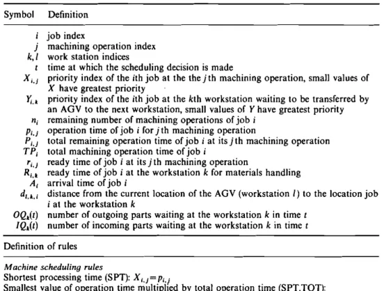
This paper attempts to provide a better understanding or scheduling problems for FMS by testing the performance of FMS scheduling rules for a wide variety of experimental conditions. Since only the machines and materials handling aspects of an FMS are under study, the scheduling rules are classified into: (I) machine scheduling rules and (2) AGV scheduling rules. The list of rules studied is presented in Table 1. The machine scheduling rules are those which are used to select the next job lrom the input queue upon the completion of the previous operation. The second group of scheduling rules are those which are used to schedule the AGVs. The machine scheduling rules were selected from recent FMS and job-shop literature. Among the AGV rules, FCFS, STD, and LOQS were already tested by Egbelu and Tanchoco (1984). The remaining AGV rules, LQS, LWKR, and FOPNR, were, therefore, included in this paper. Each of these AGV rules has unique characteristics. FCFS has the ability to complement the machine scheduling rules by serving a workcentre with the earliest job completion. This rule may easily reduce the FMS scheduling problem to a type of job shop scheduling problem if there is sufficient queue capacity, and if at the same time, the AGV speed is very high. LOQS and LQS are rules which use information on queue level at workcentres. LOQS rule assigns the AGV to the station with largest outgoing parts. This rule can be very effective if incoming and outgoing parts wait in separate queues. On the other hand, LQS selects the workcentre with the, largest overall queue level. Similarly, this rule may be very effective if both incoming and outgoing parts share the same queue. The STD rule minimizes the distance
1620 Symbol j k,I t X,.} ~.l n, Pi.}
r.,
TPi r., Ri •• Ai d'.'.i OQ.(t) IQ.(t)1. Sabuncuoqlu and D. L. Hommertzheim
Definition job index
machining operation index work station indices
time at which the scheduling decision is made
priority index of the ith job at the thejth machining operation, small values of X have greatest priority
priority index of the ith job at the kth workstation waiting to be transferred by an AGV to the next workstation, small values of Yhave greatest priority remaining number of machining operations of job i
operation time of job i forjth machining operation
total remaining operation time of job i at itsjth machining operation total machining operation time of job i
ready time of job i at itsjth machining operation
ready time of job i at the workstation k for materials handling arrival time of job i
distance from the current location of the AGV (workstation I) to the location job i at the workstation k
number of outgoing parts waiting at the workstation k in timet number of incoming parts waiting at the workstation kin time t Definition of rules
Machine scheduling rules
Shortest processing time (SPT): Xi . } = Pi.}
Smallest value of operation time multiplied by total operation time (SPT.TOT):
X,.}=Pi.}xTP,
Smallest value of operation time divided by total operation time (SPT/TOT): Xi.}=PijTPi
Largest value of operation time multiplied by total operation time (LPT.TOT): X,.}= -Pi.}x TPi
Largest value of operation time divided by total operation time (LPT/TOT): X i.}= -P,jTPi
Least work remaining (LWKR): X,.}=P,.} Most work remaining (MWKR): X i.}= -Pi.}
Fewest number of operations remaining (FOPNR): X,.}= n, Most number of operations remaining (MOPNR): Xi . } = - n, First come first served (FCFS): X,.}= ri . }
First arrived first served (FAFS): Xi.}=A, RANDOM (job priority is random) AGV scheduling rules
First come first served (FCFS):
li.•
=
R,.•Largest output queue size (LOQS):
li.•
= -
OQ.(l)Shortest travelling distance (STD):
li.•
=d,.'.iLargest queue size (LQS), including incoming and outgoing parts:
li.•
=
-(OQ.(t)+ IQ.(I))Most work remaining (MWKR):
li.•
= - Pi.}Fewest number of operations remaining (FOPNR): li .•
=n,
travelled. Its performance depends upon the particular layout, however, it may speed up the circulation of parts on the shop floor. LWKR and FOPNR rules are the only ones which set the priority of AGVs by using part information.
3. System considerations and simulation model
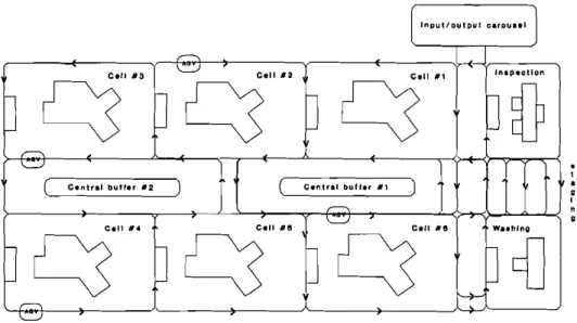
Figure I shows the layout of the hypothetical FMS studied and reported in this paper. There are eight workstations. Six of these workstations are typical machining centres which perform a wide variety of operations, such as turning, milling, and drilling. The two remaining stations are used for washing and inspection. Each workcentre has a limited input/output buffer queue in which parts can wait before and , after an operation. In addition, there is an input/output carousel where parts are mounted/demounted to fixtures and palletized for transfer. The arriving parts are held in the carousel and allowed into the system on FCFS basis as long as both an AGV and one queue space at the destination workcentre are available. There are also two central buffer areas at which parts are temporarily stored to prevent system locking or when the destination station queue is full for a part travelling to this station. Materials and parts are transferred in the system by an AGV system. Each AGV moves a part between the workcentres along a predetermined path. This path (material flow)is assumed to be unidirectional. Upon the completion of a part transfer, an idle AGV either returns to the staging area or stays at the same station for the next journey depending upon the' current operating policy. As far as the link between the workstations and the AGVs is ' concerned, a 'direct access part retrieval design' is considered to be operational. Therefore, any part from the queue can be retrieved regardless of its position in the queue. The FMS described above is a hypothetical system. The purpose of developing such a system is to use it as a 'test-bed' to measure performances of algorithms for design and operation of FMS. It was designed by considering several existing FMS configurations. A SIMAN (Pegden 1985)discrete simulation model was developed to
[ ," •• tto.,,", " '. . . . ,
J
r-r-;
Cell "3 '-=.) Cell112 Cell #1 Inlpecllon
]
q oq
0
q
DO
,---,
<:»
( Central burr.r "2 ) ( C"ntral bull.r #1 )
,---,
Cell 114 Cell #15 <:» Cell Ie W•• llino
~q
Jq
0
q
Jq]
,---, ~
'-=.)
1622 I. Sabuncuoglu and D.L. Hommertzheim
represent the FMS. In the development stage, CINEMA (Healy 1986), an animation package, was also used to verify the control logic.
Blocking and locking are two critical problems of any capacitated system such as an FMS. Blocking occurs when a machine can not move its part to a queue (buffer) area because the queue is full. Consequently, a part can not proceed to the next station nor can the affected machine be released. This in turn causes starvation of some other resources and reduces the system efficiency. Similarly, an AGV can also be blocked by another AGV if there is high traffic congestion in a system.
Locking occurs when the system is totally prevented from functioning. This occurs when one or more queues at workcentres are full and the affected machines are blocked at the same time. Thus, no part movement can be achieved. In general, the locking phenomenon depends upon the design of the system as well as its current status and operating policies. In any case, a mechanism to prevent it from occurring is required. In the system considered, the following preventive scheme was used:
(I) Since a common buffer area is used for both incoming and outgoing parts at each workcentre, the number of incoming parts in the queue is limited to one less than the queue capacity. Thus, a part finishing an operation can obtain queue space as long as the queue is not full with other outgoing parts. (2) Upon job completion at any work centre, if the machine is blocked and there is
an AGV available then one of the outgoing parts at this workcentre is transferred to a central buffer area.
(3) Similarly, upon the completion of any materiaJ transfer, an AGV checks possible blocking and locking conditions in the system.Ifthere is one, then it moves a part from the problem area to a central buffer.
4. Experimental conditionsandassumptions
The simulation model described in the previous section is rather general and requires significant computation time to perform the experimental studies. Therefore, some simplifying assumptions were made. These assumptions together with some other operational policies are as follows:
(J) Each workcentre can handle at most one operation at a time and each machine and AGV is continuously operational without any breakdown.
(2) Pre-emption is not allowed and set up time is included in the operation time. (3) Whenever a machine and an AGV become idle, the next job in the queue is
processed immediately (i.e. non-delay scheduling).
(4) Partload/unload time to and from an AGV is taken as a constant. Part transfer time by an AGV is directJy proportional to the distance travelled (AGV speed is constant).
(5) Buffer capacity at each workcentre is limited and equal. Thus, a part completing a current operation waits in the queue at the workcentre until the next station queue and an AGV are available. There are no capacity restrictions on the central buffer area and the input/output carousel.
(6) An AGV transfers only one part at a time (i.e. unit load is one). At intersections in the AGV path network (Fig. I) an AGV moving a part has priority over other AGVs travelling empty. In case ofa tie, the right of passing at the intersection is determined on a FCFS basis.
(7) Upon job completion at any workcentre, if there is more than one AGV available to transfer the part to the next station, the one closest to the workcentre which is demanding service is selected.
(8) The tooling system is not modelled and an infinite number of pallets is assumed.
The purpose of this study is to analyse the FMS scheduling problem by taking into account the limited capacities of not only the machines but also the materials handling system and the in-process inventory. Therefore, the simulation model is developed in such a way that these three resources and their interactions are represented in detail. Furthermore, in some ways, the system described above can be viewed as an extended job-shop in which machining centres have limited input/output buffer capacities and are tied together with an AGV materials handling system.
Data for the simulation runs were generated by stochastic variables in a subprogram written in FORTRAN. The job interarrival time was exponentially distributed. Each job was processed by a series of workcentres. The number of operations (number of machines to visit) was determined by a discrete uniform distribution between one and six. The machine assignment was random and no job was allowed to visit the same machine more than once. As a result, machine loads were kept equal. Besides the workcentres, all jobs visited the washing station. However, only 50% of the jobs were processed by the inspection station. In the simulation experiments,
only two AGVs were employed. The reason for using a small number of AGVs is that the simulation execution time increased significantly when a large number of AGVs was operated. The scheduling rules were tested under the following experimental conditions:
• varying machine and AGV load levels; • different queue capacities;
• varying AGV speeds.
For the operation time distribution, a normal distribution was used and only the positive values were considered. There are three reasons· for using the normal distribution for generating operation times. First, the normal distribution is one of the distributions for which the variance is independent of mean. This allows the analyst to check the effects of the processing time variance on the relative performance of some scheduling rules. Second, in computer-integrated manufacturing environments such as FMSs, the variability in operation times can be greatly reduced by appropriate process planning and the loading decision which is made prior to scheduling. Third, as noticed by some researchers such as Wilhelm (1987), total batch processing times can be (approximately) normally distributed.
When compared with a traditional job shop, statistical analysis of simulation output of an FMS environment is more difficult because of blocking/locking problems. and continuous changes in the characteristics of the system.In practice, an FMS has to
deal with relatively low production volumes with greater product variety. This production variability coupled with multi-resource interactions and blocking/locking problems makes it very difficult to analyse the system steady-state behaviour. Indeed, stochastic processes for real FMS may not have a steady-state distribution. Thus, these systems require a considerable amount of computer time to identify and estimate their true steady-state performance characteristics (if they exist).In the hypothetical FMS
1624 1. Sabuncuoqlu and D.L. Hommertzheim
to be static. Furthermore, a preventive scheme discussed in the previous section was very effective in dealing with blocking/locking. Thus, it was expected that such a simplified system would have a steady-state response. Analyses of the initial transient state based on some pilot simulation runs confirmed our expectation.
Since the objective was to measure the relative performance of alternative rules or operating policies, it was logical to compare them under identical conditions. The use of a common random number variance reduction scheme ensured that each job arrived at the same time and was assigned the same routeing and operation times for each case considered (the variance reduction scheme allows comparisons with shorter run times). Another problem encountered in simulation experiments is specifying the contents of a sample drawn from the system (i.e. deciding on which jobs to include in the sample in measuring relative performance alternatives). A scheme suggested by Conway (1963) was utilized. In each experiment, the jobs were numbered in the order of their arrival and the flow-times were measured accordingly. Specifically, based on some pilot runs, the statistics for the first 300jobs were discarded and the sample was collected for only the jobs numbered between 301 and 3300. (Pilot runs were conducted to select an appropriate number of jobs for the runs).
5. Analysis of simulation results
5.1. Performance of scheduling rules with respect to elements of mean flow-time Before comparison was made of scheduling rules under varying experimental conditions, the relative performance of scheduling rules were compared against the components of the mean flow-time. The flow-time of a job is the total time that a job spends in the system and can be expressed as follows:
flow-time
=
total processing time+ total waiting time in load/unload area + total waiting time in in-shuttle + total waiting time in out-shuttle
+ total transportation (or materials handling) time
+set up and load/unload time (I)
Mean flow-time (MF) is the average of the flow-times of all jobs measured during a simulation run.
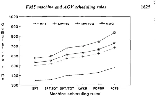
MF criterion is used primarily because it is a very critical indicator of the lead time and it also provides important information that can be used for setting the due-dates or due-date allowances (Sabuncuoglu and Hommertzheim 1990). Moreover, it is proportional to the work-in-process levels. Thus, in various industrial applications, practitioners usually try to minimize the average time in the system. Since in this study, the set up time is included in the processing time, or at least it is assumed to be sequence independent and the total processing time is constant (predetermined upon arrival of job), the only way to minimize the mean flow-time is to reduce the waiting times.Itwas expected that machine scheduling rules would affect waiting time in the in-shuttle, and AGV scheduling rules would affect waiting time in the out-shuttle. Finally, the combinations of machine and AGV scheduling rules would affect the waiting time in the loading/unloading area. To test these conjectures, pilot simulation runs were made. Figures 2 and 3 are cumulative graphs which present mean flow-times and their
1000 C 900 u m u 800 I a 700 t ; v 600 e t 500 i 400 [ m e 300
- MFT +.MWTIO -l<- MWTOO -e-MWC
SPT SPT.TOT SPTITOT LWKR FOPNR FCFS
Machine scheduling rules
Figure 2. Mean flow-time and its principal elements for some machine scheduling rules.
1000 , - - - ,
c
u m u I a t i v e- MFT + MWTlO -l<- MWTOO -e-MWC
t i m e 500 400 300 '---_ _L - _ - - - - ' ' - - _ - - '_ _---<_ _---'-_ _---'-_ _---"
LOS SOT LWKR FOPNR LOOS FCFS
AGV scheduling rules
Figure 3. Mean flow-time and its principal elements for some AGV scheduling rules.
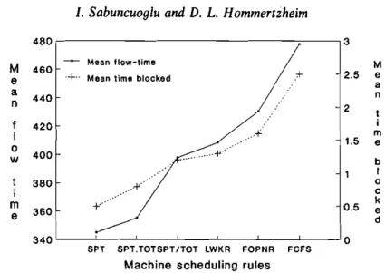
principal components as a function of scheduling rules used.Ingeneral, the elements of mean flow-time increase in the same order as the flow-time.Inother words, a rule which minimizes mean waiting time in input queue (MWTIQ), mean waiting time in output queue (MWTOQ), or mean waiting time in carousel (MWTC) also yields a better mean flow-time performance. Furthermore, the rules which were very effective in preventing' blocking also minimize the mean flow-time (Figs 4 and 5).These results indicate that if a method could be found to minimize one of the waiting time components and the number of blockings, this would probably reduce mean flow-time. Combination of the SPTand LQS machine and AGV scheduling rules exhibited the best reduction in mean flow-time and the various elements that constitute it.
5.2. Mean flow-time performance of scheduling rules at varying machine and AGV load conditions
Setting machine and AGV load levels was another problem in this research.Inthe traditional job-shop studies, the materials handling aspect of the system is usually,
1626 I. Sabuncuoglu and D.L. Hommertzheim
480 3
M 460 Mean flow-time 2.5 Me
e +. Mean time blocked
a a 440 n n 2 I f 420 i I 1.5 me 0 400 W b I t 380 0 i .... c . ' k m 360 +., 0.5 e e d 340 0 SPT SPT.TOTSPT/TOT LWKR FOPNR FCFS
Machine scheduling rules
Figure 4. Mean flow-lime and mean time blocked for some machine scheduling rules.
T o I a I n u m b e r 480 Mean t1ow·time M 460 +. No. of blackings e 530 a 440 n f 420 430 I
*
0 W 400 330 t 380 .+ i m .. 230 e 360 340 130 o f b I o c k i nLOS SOT LWKR FOPNR LOOS FCFS ~
AGV scheduling rules
Figure 5. Mean flow-lime and lotal number of blockings for some AGV scheduling rules.
ignored; the arrival rate is used to change the machine or the system load level. But, in a capacitated system such as an FMS, this would dramatically affect the load level ofthe AGY subsystem as the arrival rate determines the demand rate of the materials handling system. Another way of changing the machine load levels without dramati-cally affecting the AGY load levels is to control operation time distribution parameters. In this case, there are two choices: (I) correlate the variance with the mean so that the coefficient of variation (CY) is the same across load levels, or (2) use the same variance but a different CY for each load level. In the simulation experiments, these three methods were used to set load levels. However, in most of the discussions presented here, the results of the former method will be reported.
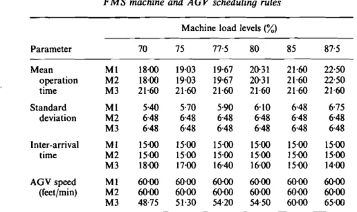
The values of input parameters for each method are given in Table 2. These parameter values were determined based on pilot simulation experiments so that the average machine and AGY load levels are similar in each case.
Machine load levels(%) Parameter 70 75 77-5 80 85 87·5 Mean M1 18·00 19·03 19-67 20·31 21·60 22·50 operation M2 18·00 19·03 19·67 20·31 21·60 22·50 time M3 21·60 21·60 21·60 21·60 21·60 21·60 Standard MI 5·40 5·70 5·90 6·\0 6'48 6·75 deviation M2 6'48 6'48 6'48 6·48 6·48 6·48 M3 6·48 6·48 6·48 6·48 6·48 6·48 Inter-arrival MI 15·00 15·00 15·00 15·00 15·00 15·00 time M2 15·00 15·00 15·00 15·00 15·00 15·00 M3 18·00 \7·00 16·40 16·00 15·00 14'00 AGV speed MI 60'00 60·00 6Q-00 60'00 60·00 6Q-00 (feet/min) M2 60·00 6Q-00 60·00 6Q-00 60·00 60·00 M3 48·75 51·30 54·20 54·50 60·00 65·00
Nomenclature: M 1, mean flow-time results based on the first method (changing processing times) using the same coefficient of variation; M2, mean flow-time results based on the first method using the same variance; M3, mean flow-time results based on the second method (changing arrival rate).
Table 2. Input parameters for simulation experiments for normally distributed processing times.
Although the objective was to test the performance of the scheduling rules under varying load levels, it is worthwhile discussing the effect of three different methods of setting average load level on mean flow-time.
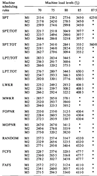
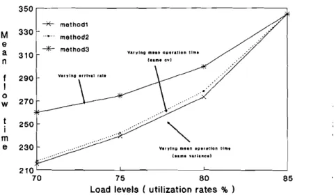
The mean flow-time performances of the rules under each load level are depicted in Table 3. In these simulation experiments, FCFS was used as the AGV scheduling rule. Figure 6 shows the mean flow-time performance of SPT under the three methods.Itis clear that the first two methods produce similar results. However, the third method was quite different. At the lower load levels (i.e. 70 and 75%), differences between the methods were greatest but they prod uced similar performance at the standard condition (i.e. 85% load level). This type of behaviour for the methods can be explained in conjunction with Table 2. As can be seen in Table 2, the mean and standard deviation of processing times are relatively high for the last two methods over the ranges in which machine loads were varied. Thus, it is reasonable to expect higher flow-time performances with the last two methods. This result does not mean that the first method always achieves lower flow-times performances.Itdepends rather on the where the standard conditions are set initially. Ifthey were set at lower values of machine utilization, the performances of the method would be different.
As can be seen in Table 3, the relative effectiveness of rules became accentuated under highly loaded shop conditions irrespective of the way of setting machine load levels.Itis interesting that SPT.TOT and SPT are the only two rules that did not allow the system to saturate at the very high utilization level (i.e.90%).At this rate, SPT.TOT performed much better than the SPT rule. However, at the other load conditions, SPT is still preferred. Finally, as can be observed from Table 3, these rules are followed by LWKR and FOPNR. Other rules performed poorly.
There are also at least two ways to control the load levels of the AGV system. The first method is simply to change the AGV service rate by changing the AGV speed. The
1628 1. Sabuncuoqlu and D.L. Hommertzheim
Machine Machine load levels(%)
scheduling rules 70 75 80 85 87·5 SPT MI 215·4 239·2 273·6 345·0 625·0 M2 217·8 242·0 278·5 345·0
•
M3 259·9 274·6 299·8 345·0•
SPT/TOT MI 221·7 251·8 304·9 397·7•
M2 223·7 249·6 298·0 397·7•
M3 268·6 286·8 325·8 397·7•
SPT.TOT MI 216·7 241·0 284'1 355·2 560·8 M2 219·1 246·0 282-4 355·2•
M3 262·7 279-6 309·4 355'2•
LPT/TOT MI 283-3 283-4 344·5•
•
M2 256·3 291·7 368·6•
•
M3 286·0 320·2 375·3•
•
LPT.TOT Ml 276·7 280·7 344·5 650'3•
M2 254·7 293·3 366·3 650·3•
M3 292·0 330·1 377-6 650·3•
LWKR MI 225·2 249·2 293·2 408·3•
M2 228·1 259·7 308·2 408·3•
M3 266·2 292-4 322·2 408·3•
MWKR MI . 285·7 285·8 378·1•
•
M2 252·0 293·7 394·0•
•
M3 294·0 325·3 395·2•
•
FOPNR MI 255·0 255·0 312·5 430·4•
M2 228·4 26(}5 312·0 430·4•
M3 272-3 293-9 330·7 430·4•
MOPNR MI 267·0 267·0 341·2•
•
M2 240·6 276·8 355·9•
•
M3 275·0 320·2 382·0•
•
RANDOM MI 257·3 257·4 314·7 432·0•
M2 232'9 265'6 323·5 432·0•
M3 277-1 293-8 340-4 432·0•
FCFS MI 228·7 257-6 320·5 477-7•
M2 236·0 265·5 316·8 477·7•
M3 278·2 302·7 343-8 477-7•
FAFS MI 257·2 257·2 312·4 411·0•
M2 234·1 260·0 305·7 411·0•
M3 271·5 294·3 334·0 411·0•
M I, Mean flow-time results based on the first method (changing processing times) using the same coefficient of variation; M2, mean flow-time results based on the first method using the same variance; M3, mean, flow-time results based on the second method (changing arrival rate).
• System is saturated.
Table3. Mean flow-time performance of the machine scheduling rules at varying machine load levels (FCFS is used as the AGV scheduling rule).
alternative method is to change the average number of operations per arrival. While the former method does not affect machine load, the second method may dramatically affect machine utilization as the average total work content changes per arrival under the same machining service rate. Therefore, the former method was utilized in the simulation experiments. The AGV speed was tested at 75, 70, and 60 feet/min corresponding to average AGV utilizations of 73,77, and 88%, respectively. The AGV utilization changed slightly depending upon the relative effectiveness of the rule.
The results of the simulation experiments are summarized in Table 4. They indicate that LQS is the preferred AGV rule and this is followed by the LWKR and STD rules. L WKR Displayed a slightly better flow-time performance than STD. The other rules did not perform well compared to these three rules. Finally, as was expected, the relative performances or rules became more significant as the AGV load or utilization increased. When considering variances on flow-times, it was generally observed in simulation experiments that mean and variance of the flow-times are correlated (i.e. a rule with larger mean flow-time value resulted in larger variance). There were some exceptions with the SPT rule at large queue capacities.
At this stage, STD and LQS were further compared at varying load levels. Since the AGV rule LWKR performed competitively with these rules, it was also included in the
350 ""*- method1 M 330 ... method2 e --*" a method3 310 n f 290 I 0 W 270 t 250 i m e 230 210 70
Va.,lng 1lI•• n opI •• llon Hili.
( •• ml~arl."c:.1
75 80
Load levels ( utilization rates % )
85
Figure 6. Mean flow-time performance of SPT under varying load levels.
AGV Average load level of AGV system(%) scheduling rules 73 77 88 FCFS 407·6 424·0 477-7 STO 393-9 415·2 413·5 LOQS 400·5 441·4 445·8 LQS 372-8 372-0 388·7 LWKR 383'0 412·0 438·9 FOPNR 420-2 430·4 454·3
Table4. Mean flow-time performance of the AGVscheduling rulesat varyingAGVutilization rates (FCFS is used as the machine scheduling rule).
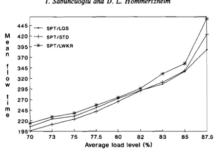
1630 I. Sabuncuoglu and D.L. Hommertzheim 445 - SPTILOS M 420 -+- SPTISTD e --*-SPT ILWKR a 395 n 370 f 345 I 0 320 W 295 t 270 i m 245 e 195¥'---'---'---'---'---'---L----'---70 73 n 77.5 80 82 83 85 8~
Average load level(%)
Figure 7. Performance of STD, LQS, and LWKR with SPT at varying machine load levels.
87.5 85
75 77.5 80 82 83
Average load level(%) 73 - SPT.TOTILOS -+- SPT.TOTISTD -+- SPT.TOTILWKR 270 220 195"---'---'---'---'---'---L---'---70 370 345 320 395 f I o W 295 t i m 245 e M 420 e a n 445
Figure 8. Performance of STD, LQS, and LWKR with SPT.TOT at varying machine load levels.
simulation experiments. Recall that each ofthese rules has different characteristics. The LWKR uses job related information to prioritize AGVs. The LQS rule utilizes the queue level information and is very effectivefor reducing the number of blockings; STD priority assignment depends on the AGV network (or layout) rather than job related information and queue levels. Two machine scheduling rules.Sl'Tand SPT.TOT, were considered in the experiments because they were found to be the best machine scheduling rules for all of the experimental conditions tested so far. The simulation results are depicted in Figs 7 and8. They show the mean flow-time performances of rules. As can be seen in the figures, STD and LQS performed better than LWKR. The STD rule produced slightly better mean flow-time performance than LQS at the low or moderately loaded shop conditions irrespective of the machine rule combination. However, LQS began to show better performances than STD when the machine load increased (i.e. above the 80% utilization level).
At low and moderately loaded conditions, where blocking was less probable, STD minimized the AGV queue by minimizing the distance travelled. However, as the load was increased, blocking increased, and eventually the LQS rule, which was very sensitive to blocking, began showing better performances than STD. From the relative performance of AGV rule LWKR, it is clear that job related information did not provide sufficient flow-time improvements over the other type of information that STD and LQS utilize.
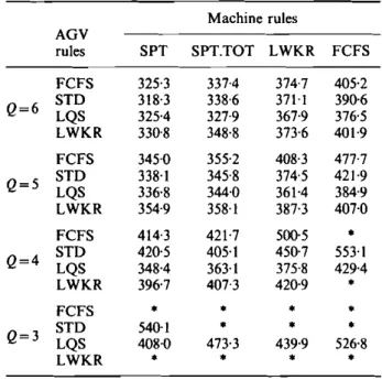
5.3. Relative performance of the machine and AG V scheduling rules at varying queue capacities
The effect of different queue capacities on the relative performances of scheduling rules was also investigated in this study. The mean flow-time performances of four machine and AGV scheduling rule combinations at varying queue capacities are summarized in Table 5. Recall that under the standard experimental condition, the queue capacity was five. In general, SPT still provided a substantial flow-time improvement over the other machine scheduling rules, such as SPT.TOT, LWKR, and FCFS when the queue capacity was reduced. Similarly, LQS was a very effective AGV scheduling rule at the smaller queue capacities. As can be seen in Table 5, there was an interaction between AGV rules-FCFS, STD-and machine rules-SPT, SPT.TOT-when Q=4. It can also be seen in the bottom part of the Table 5 that the system saturated for some rule combinations when the queue size was three (Q=3). Only the machine scheduling rules with the LQS combination did not saturate at that queue capacity level. Similarly, LQS was a very effective AGV scheduling rule at the smaller
Machine rules AGV rules SPT SPT.TOT LWKR FCFS FCFS 325-3 337-4 374·7 405·2 Q=6 STOLQS 318·3325·4 338·6327-9 37\-1367-9 390·6376·5 LWKR 330·8 348·8 373-6 401·9 FCFS 345·0 355'2 408·3 477-7 Q=5 STOLQS 338·1336·8 345·8344·0 374·5361·4 421·9384'9 LWKR 354·9 358·1 38703 407·0 FCFS 414·3 421·7 500·5
•
Q=4 STOLQS 420·5348·4 405·1 450·7 553·1 36H 375·8 429·4 LWKR 396'7 40703 420·9•
FCFS•
•
•
•
STO 540·1•
•
•
Q=3 LQS 408·0 473-3 439·9 526·8 LWKR•
•
•
•
• System was saturated.
1System was saturated at Q=2 for all rule combinations.
Table 5. Mean flow-time performance of machine and AGV scheduling rules at varying queue capacities.1
1632 I. Sabuncuoglu and D.L. Hommertzheim
queue capacities. Again, only the machine scheduling rules with the LQS combination did not saturate at that queue capacity level.
With the limited queue capacities, buffer space at each workcentre was one of the scare resources in the system. That is, upon the completion of a current operation, a part did not only have to seize an AGV but had to also find an available space at the next workcentre before it arrived there. Therefore, in such systems, the queue level was an important factor for the system performance. In fact, the results of simulation experiments indicated that SPT/LQS was the best rule combination as the capacity of queues is reduced. This is not surprising since the AGV rule LQS is very sensitive to the queue capacity and at the same time, SPT is a very effective machine scheduling rule which usually minimizes the average queue time. Thus, the combination of these two rules minimized the number of blockings, circulated the parts faster, and consequently, achieved the lowest mean flow-time performance.
As can be seen from the Table 5, the system was saturated at the low queue capacities. Later, in order to obtain a better understanding of the performances of the rules at low queue capacities, the original machine load level was decreased from85%
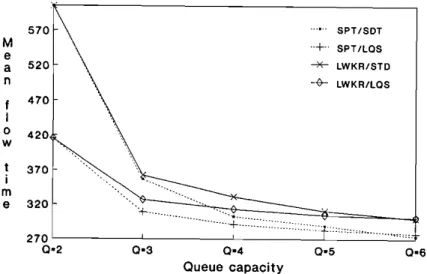
to82%by reducing the values of the operation time parameters. The mean and variance of the operation time distribution were taken as20·96 and 6,29, respectively. Similarly, the AGV load was reduced by increasing the AGV speed from60 to 75 feet/min. Based on the previous performances of the rules, six different- rule combinations were considered. These were SPT, SPT.TOT, and LWKR for the machine scheduling and STD and LQS for AGV scheduling, respectively. The simulation model was run under this new experimental condition and the mean flow-time performances at varying queue capacities are shown in Fig.9.
In general, the machine scheduling rule SPT still provided flow-time improvements
over the LWKR rule regardless of the combination with AGV scheduling rules. Similarly, LQS performed better than STD when the queue capacity was reduced.Itis interesting to note that both of the machine scheduling rules produced similar performances when the queue capacity was two. At this queue capacity, however, the
::::::::.",
...
...,,:.. SPT/SOT .-+.. SPTILOS"*'
LWKRISTD -4- LWKR/LOS M e a n f I 0 420 w t 370 i m e 320 270 0-2 0-4 Queue capacity 0-5 0-6performances ofthe AGV rules were quite different. In the simulation model, due to the type of preventive scheme used for blocking, there can be at most one incoming part in any queue when the queue capacity is two. Unfortunately, with no queues or one part in the queue, there are no decision possibilities to improve the mean flow-time. However, this does not mean that the scheduling decision is not likely tobecritical as indicated by Co et aI. (1988) who investigated the effect of short queue lengths on the relative performance of scheduling rules. But it indicates that in short queue length systems such as an FMS, scheduling of materials handling equipment (including AGVs) and sequencing of part loading at an input/output carousel may become more critical. Thus, the scheduling decision in an FMS is still as important as in a job-shop.
Tn a typical FMS, both the machining centres and the AGV system are closely integrated as the outputs from one subsystem are the inputs to the other subsystem. Because of these interactions, both can influence the flow of jobs at any time in the system. At one time machining centres can be the constrained resource whereas, at another time, the AGV system becomes a critical resource or 'a driving force' for the material flow and eventually dominates the schedule. Thus the performances of the rules when the queue capacity is two (Fig. 9)show that for the case in which the machine scheduling rules are not able to improve the mean flow-time due to a lack of decision opportunities in the short queue length situations, a better method of scheduling the AGVs can, in fact, improve the mean flow-time significantly. This result also strengthens the previous conjecture about the importance of scheduling decisions in an FMS.
6. Concluding remarks and suggestion for further research
This paper addressed the FMS scheduling problem by comparing the mean flow-time performance of different machine and AGV scheduling rules using a simulation model. The results indicated that at high utilization rates, in which most FMS usually operate, the way that machines and AGVs are scheduled can significantly affect the system performance. Therefore, not only machines but also AGVs should be scheduled in the most effective way. The results can besummarized as follows:
(I) As the machine and AGV loads (or utilizations) increase, the mean flow-time increases.
(2) Mean flow-time is also very sensitive to the variance of the operation time distribution.
(3) As the machine and/or AGV loads increase, differences in the performance of the scheduling rules for the mean flow-time criterion become more significant. This is because, as the utilization of the system increases, the number of parts waiting in the queues increases and eventually the superior rules have an opportunity to improve the flow-time performances significantly.
(4) Among the machine scheduling rules tested against the mean flow-time criterion, SPT and SPT.TOT appeared to be the best rules with any combination of AGV rules. In most of the cases, SPT performed better than SPT.TOT. In the other cases, the SPT.TOT rule displayed better mean flow-time performance with the FCFS machine rule combination at high utilization rates. These two rules were followed by SPT/TOT and LWKR.Itis interesting to note that the FO PNR rule did not perform well either as the machine or the AGV scheduling rule. Also, FAFS produced better performances than FCFS. Among the AGV rules tested, STD and LQS were the best AGV rules with any machine scheduling rule combination.
1634 I. Sabuncuoglu and D.L. Hommertzheim
(5) When the queue capacities were reduced, the system experienced higher flow-times due to the increase in the number of blockings and the additional travel of the AGVs to the central buffer area. Furthermore, at very low queue capacity (i.e.
Q
=2),all the machine scheduling rules produced the same mean flow-time performances due to a lack of decision possibilities in short queue length situations. However, the perfor-mances of the AGV rules were quite different under these conditions. Especially, LQS improved the mean flow-time significantly. In fact, LQS always dominated the STD rule when the queue capacities were decreased.The results presented in this paper should be interpreted with reference to the hypothetical (or example) FMS and the experimental conditions described earlier. Realizing that each FMS is custom made, there is a need for further research to develop new rules and continue testing the existing ones under different FMS configurations and experimental conditions against various performance criteria. One such experi-mental condition could be varying system characteristics such as arrival rates, processing time parameters, and the number of AGVs operating. Only the mean flow-time performance measure was considered in this paper while due-dates and performance of rules against due-date related measures also have great importance for future work.
References
ACREE, E. S., and SMITH, M. L., 1985, Simulation of a flexible manufacturing
system-applications of computer operating system techniques. The 18th Annual Simulation
Symposium, 205-216. IEEE Computer Society Press, Tampa, Florida.
BLACKSTONE, J. H., PHILLIPS, D. T., and HOGG, G. L., 1982, A state-of-the-art survey of
dispatching rules for manufacturing job shop operations. International Journal of
Production Research,20(I),27-45.
BROWNE, J., RATHMILL, K., SETHI, K., and STECKE, K., 1984, Classification of flexible
manufacturing systems. The FMS Magazine, April, 114-117.
BUZACOTT, J. A., and YAO, D. D., 1985, Flexible manufacturing systems: a review of analytical
models.Management Science,32 (7), 890-905.
CHOI, R. H., and MALSTROM, E. M., 1988, Evaluation of traditional work scheduling rules in a
flexible manufacturing system with a physical simulator. Journal of Manufacturing
Systems,7(1), 33-45.
Co, H. C,JAW, T.1.,and CHEN, S. K., 1988, Sequencing in flexible manufacturing systems and other short queue-length systems. Journal of Manufacturing Systems, 7 (I), 1-7. CONWAY, R. W., 1963, Some tactical problems in digital simulation.Management Science,10(l),
47-61.
CONWAY, R. W., MAXWELL, W. L., and MILLER, L. W., 1967,Theory of Scheduling (Reading,
Mass.: Addison-Wesley).
DENZLER, D. R., and BOE, W. J., 1987, Experimental investigation of flexible manufacturing system scheduling rules. International Journal of Production Research,25 (7), 979-994.
DUPONT, G. C, 1982, A survey of flexible manufacturing systems. Journal of Manufacturing
Systems, 1 (I), 1-16.
EGBELU, P. J., 1987, Pull versus push strategy for automated guided vehicle load movement in a
batch manufacturing system.Journal of Manufacturing Systems, 6 (3), 209-221.
EGBELU, P. J., and TANCHOCO, J. M. A., 1984, Characterization of automated guided vehicle dispatching rules. International Journal of Production Research,22 (3), 359-374.
GROOVER, M. P., 1987,Automation, Production Systems and Computer Integrated Manufacturing
(New York: Prentice-Hall).
HEALY, K. J., 1986, Cinema tutorial.Proceedings of 1986 Winter Simulation Conference, 207-211.
Society of Computer Simulation, San Diego, California.
KING, J. R., 1979, Scheduling and the problem of computational complexity. Omega,7 (3),
KIRAN, A. S., and SMITH, M.L.,1984a, Simulation studies in job shop scheduling-a survey. Computers and Industrial Engineering, 8 (2), 87-93.
KIRAN, A. S., and SMITH, M.L.,1984 b, Simulation studies injob shop scheduling-performance of priority rules. Computers and Industrial Engineering, 8 (2), 95-105.
KUSIAK, A., 1985, Flexible manufacturing systems: a structural approach.International Journal of Production Research, 23 (6), 1057-1074.
KUSIAK, A., 1986a, Applications of operational research models and techniques in flexible manufacturing systems. European Journal of Operations Research, 24 (2), 336-345. KUSIAK, A., 1986 b, Scheduling flexible machining and assembly system. In K. E. Stecke and R.
Suri (eds),Proceedings ofthe Second ORSA/T1 MS Conference on Flexible Manufacturing Systems: Operations Research Models and Applications, 521-526. Elsevier Science Publishers B.V., Amsterdam.
KUSIAK, A., and CHEN, M., 1988, Expert systems for planning and scheduling manufacturing systems. European Journal of Operations Research, 34 (3), 113-130.
MONTAZERI, M., and VAN WASSENHOVE, L. N., 1990, Analysis of scheduling rules for an
FMS. International Journal of Production Research, 28 (4), 785-802.
PANWALKAR, S. S., and ISKANDER, W., 1977, A survey of scheduling rules.Operations Research, 25 (1),45-61.
PEGDEN, C. D., 1985,Introduction to SIMAN (State College, Pennsylvania: Systems Modeling Corporation).
RAMAN, N., TALBOT, F. B., and RACHAMADUGU, R. V., 1986, Simultaneous scheduling of machines and material handling devices in automated manufacturing. In K. E. Stecke and R. Suri (eds),Proceedings ofthe Second ORSA/T1MS Conference on Flexible Manufactur-ing Systems: Operations Research Models and Applications, 321-332. Elsevier Science Publishers BY, Amsterdam.
SABUNCUOGLU, 1., and HOMMERTZHEIM, D., 1989a, An Investigation of Machine and AGV scheduling rules in an FMS. InK. E. Stecke and R. Suri (eds),Proceedings of the Third ORSA/TI MS Conference on Flexible Manufacturing Systems: Operations Research Models and Applications, 261-266. Elsevier Science Publishers B.V., Amsterdam. SABUNCUOGLU, I., and HOMMERTZHEIM, D., 1989 b, Expert simulation systems-recent
develop-ments and applications in flexible manufacturing systems. Computers and Industrial Engineering, 16 (4), 575-585.
SABUNCUOGLU, 1., and HOMMERTZHEIM, D., 1990, An Investigation of the FMS due-date scheduling problem: evaluation of due-date assignment rules. Working paper: 90-102, Industrial Engineering Department, The Wichita State University.
SElDMANN, A., and TENEBAUM, A., 1986, Optimal stochastic scheduling of flexible manufacturing systems with finite buffers. In K. E. Stecke and R. Suri (eds),Proceedings of the Second ORSA/T1 MS Conference on Flexible Manufacturing Systems: Operations Research Models and Applications, 487-498. Elsevier Science Publishers BY, Amsterdam. STECKE, K. E., 1985, Design, planning, scheduling, and control problems of flexible
manufactur-ing systems. Annals of Operation Research, 3, 3-12.
STECKE, K. E., and SOLBERG, J., 1981, Loading and control policies for a flexible manufacturing system. International Journal of Production Research, 19 (5), 481-490.
SURI, R., 1985, An overview of evaluative models for flexible manufacturing systems. Annals of Operations Research, 3, 13-21.
WHITE, K. P., and ROGERS, R. V., 1990, Job-shop scheduling of the binary disjunctive formulation. International Journal of Production Research, 28 (12), 2187-2200.
WILHELM, W. E., 1987, On the normality of operation times in small-lot assembly systems: a technical note. International Journal of Production Research, 25 (1), 145-149.