published as:
Amplitude analysis of the χ_{c1}→ηπ^{+}π^{-} decays
M. Ablikim et al. (BESIII Collaboration)
Phys. Rev. D 95, 032002 — Published 13 February 2017
DOI:
10.1103/PhysRevD.95.032002
M. Ablikim1, M. N. Achasov9,e, S. Ahmed14, X. C. Ai1, O. Albayrak5, M. Albrecht4, D. J. Ambrose44,
A. Amoroso49A,49C, F. F. An1, Q. An46,a, J. Z. Bai1, O. Bakina23, R. Baldini Ferroli20A, Y. Ban31, D. W. Bennett19,
J. V. Bennett5, N. Berger22, M. Bertani20A, D. Bettoni21A, J. M. Bian43, F. Bianchi49A,49C, E. Boger23,c,
I. Boyko23, R. A. Briere5, H. Cai51, X. Cai1,a, O. Cakir40A, A. Calcaterra20A, G. F. Cao1, S. A. Cetin40B,
J. Chai49C, J. F. Chang1,a, G. Chelkov23,c,d, G. Chen1, H. S. Chen1, J. C. Chen1, M. L. Chen1,a, S. Chen41,
S. J. Chen29, X. Chen1,a, X. R. Chen26, Y. B. Chen1,a, H. P. Cheng17, X. K. Chu31, G. Cibinetto21A, H. L. Dai1,a,
J. P. Dai34, A. Dbeyssi14, D. Dedovich23, Z. Y. Deng1, A. Denig22, I. Denysenko23, M. Destefanis49A,49C,
F. De Mori49A,49C, Y. Ding27, C. Dong30, J. Dong1,a, L. Y. Dong1, M. Y. Dong1,a, Z. L. Dou29, S. X. Du53, P. F. Duan1, J. Z. Fan39, J. Fang1,a, S. S. Fang1, X. Fang46,a, Y. Fang1, R. Farinelli21A,21B, L. Fava49B,49C,
F. Feldbauer22, G. Felici20A, C. Q. Feng46,a, E. Fioravanti21A, M. Fritsch14,22, C. D. Fu1, Q. Gao1, X. L. Gao46,a,
Y. Gao39, Z. Gao46,a, I. Garzia21A, K. Goetzen10, L. Gong30, W. X. Gong1,a, W. Gradl22, M. Greco49A,49C, M. H. Gu1,a, Y. T. Gu12, Y. H. Guan1, A. Q. Guo1, L. B. Guo28, R. P. Guo1, Y. Guo1, Y. P. Guo22, Z. Haddadi25,
A. Hafner22, S. Han51, X. Q. Hao15, F. A. Harris42, K. L. He1, F. H. Heinsius4, T. Held4, Y. K. Heng1,a,
T. Holtmann4, Z. L. Hou1, C. Hu28, H. M. Hu1, J. F. Hu49A,49C, T. Hu1,a, Y. Hu1, G. S. Huang46,a, J. S. Huang15,
X. T. Huang33, X. Z. Huang29, Y. Huang29, Z. L. Huang27, T. Hussain48, W. Ikegami Andersson50, Q. Ji1,
Q. P. Ji15, X. B. Ji1, X. L. Ji1,a, L. W. Jiang51, X. S. Jiang1,a, X. Y. Jiang30, J. B. Jiao33, Z. Jiao17, D. P. Jin1,a,
S. Jin1, T. Johansson50, A. Julin43, N. Kalantar-Nayestanaki25, X. L. Kang1, X. S. Kang30, M. Kavatsyuk25,
B. C. Ke5, P. Kiese22, R. Kliemt10, B. Kloss22, O. B. Kolcu40B,h, B. Kopf4, M. Kornicer42, A. Kupsc50, W. K¨uhn24,
J. S. Lange24, M. Lara19, P. Larin14, H. Leithoff22, C. Leng49C, C. Li50, Cheng Li46,a, D. M. Li53, F. Li1,a,
F. Y. Li31, G. Li1, H. B. Li1, H. J. Li1, J. C. Li1, Jin Li32, K. Li33, K. Li13, Lei Li3, P. R. Li41, Q. Y. Li33, T. Li33,
W. D. Li1, W. G. Li1, X. L. Li33, X. N. Li1,a, X. Q. Li30, Y. B. Li2, Z. B. Li38, H. Liang46,a, Y. F. Liang36,
Y. T. Liang24, G. R. Liao11, D. X. Lin14, B. Liu34, B. J. Liu1, C. X. Liu1, D. Liu46,a, F. H. Liu35, Fang Liu1,
Feng Liu6, H. B. Liu12, H. H. Liu1, H. H. Liu16, H. M. Liu1, J. Liu1, J. B. Liu46,a, J. P. Liu51, J. Y. Liu1, K. Liu39,
K. Y. Liu27, L. D. Liu31, P. L. Liu1,a, Q. Liu41, S. B. Liu46,a, X. Liu26, Y. B. Liu30, Y. Y. Liu30, Z. A. Liu1,a,
Zhiqing Liu22, H. Loehner25, Y. F. Long31, X. C. Lou1,a,g, H. J. Lu17, J. G. Lu1,a, Y. Lu1, Y. P. Lu1,a, C. L. Luo28,
M. X. Luo52, T. Luo42, X. L. Luo1,a, X. R. Lyu41, F. C. Ma27, H. L. Ma1, L. L. Ma33, M. M. Ma1, Q. M. Ma1,
T. Ma1, X. N. Ma30, X. Y. Ma1,a, Y. M. Ma33, F. E. Maas14, M. Maggiora49A,49C, Q. A. Malik48, Y. J. Mao31,
Z. P. Mao1, S. Marcello49A,49C, J. G. Messchendorp25, G. Mezzadri21B, J. Min1,a, T. J. Min1, R. E. Mitchell19,
X. H. Mo1,a, Y. J. Mo6, C. Morales Morales14, N. Yu. Muchnoi9,e, H. Muramatsu43, P. Musiol4, Y. Nefedov23,
F. Nerling10, I. B. Nikolaev9,e, Z. Ning1,a, S. Nisar8, S. L. Niu1,a, X. Y. Niu1, S. L. Olsen32, Q. Ouyang1,a,
S. Pacetti20B, Y. Pan46,a, P. Patteri20A, M. Pelizaeus4, H. P. Peng46,a, K. Peters10,i, J. Pettersson50, J. L. Ping28,
R. G. Ping1, R. Poling43, V. Prasad1, H. R. Qi2, M. Qi29, S. Qian1,a, C. F. Qiao41, L. Q. Qin33, N. Qin51,
X. S. Qin1, Z. H. Qin1,a, J. F. Qiu1, K. H. Rashid48, C. F. Redmer22, M. Ripka22, G. Rong1, Ch. Rosner14,
X. D. Ruan12, A. Sarantsev23,f, M. Savri´e21B, C. Schnier4, K. Schoenning50, S. Schumann22, W. Shan31,
M. Shao46,a, C. P. Shen2, P. X. Shen30, X. Y. Shen1, H. Y. Sheng1, M. Shi1, W. M. Song1, X. Y. Song1,
S. Sosio49A,49C, S. Spataro49A,49C, G. X. Sun1, J. F. Sun15, S. S. Sun1, X. H. Sun1, Y. J. Sun46,a, Y. Z. Sun1,
Z. J. Sun1,a, Z. T. Sun19, C. J. Tang36, X. Tang1, I. Tapan40C, E. H. Thorndike44, M. Tiemens25, I. Uman40D,
G. S. Varner42, B. Wang30, B. L. Wang41, D. Wang31, D. Y. Wang31, K. Wang1,a, L. L. Wang1, L. S. Wang1,
M. Wang33, P. Wang1, P. L. Wang1, W. Wang1,a, W. P. Wang46,a, X. F. Wang39, Y. Wang37, Y. D. Wang14,
Y. F. Wang1,a, Y. Q. Wang22, Z. Wang1,a, Z. G. Wang1,a, Z. H. Wang46,a, Z. Y. Wang1, Z. Y. Wang1, T. Weber22,
D. H. Wei11, P. Weidenkaff22, S. P. Wen1, U. Wiedner4, M. Wolke50, L. H. Wu1, L. J. Wu1, Z. Wu1,a, L. Xia46,a,
L. G. Xia39, Y. Xia18, D. Xiao1, H. Xiao47, Z. J. Xiao28, Y. G. Xie1,a, Q. L. Xiu1,a, G. F. Xu1, J. J. Xu1, L. Xu1,
Q. J. Xu13, Q. N. Xu41, X. P. Xu37, L. Yan49A,49C, W. B. Yan46,a, W. C. Yan46,a, Y. H. Yan18, H. J. Yang34,j,
H. X. Yang1, L. Yang51, Y. X. Yang11, M. Ye1,a, M. H. Ye7, J. H. Yin1, Z. Y. You38, B. X. Yu1,a, C. X. Yu30,
J. S. Yu26, C. Z. Yuan1, W. L. Yuan29, Y. Yuan1, A. Yuncu40B,b, A. A. Zafar48, A. Zallo20A, Y. Zeng18, Z. Zeng46,a,
B. X. Zhang1, B. Y. Zhang1,a, C. Zhang29, C. C. Zhang1, D. H. Zhang1, H. H. Zhang38, H. Y. Zhang1,a, J. Zhang1,
J. J. Zhang1, J. L. Zhang1, J. Q. Zhang1, J. W. Zhang1,a, J. Y. Zhang1, J. Z. Zhang1, K. Zhang1, L. Zhang1,
S. Q. Zhang30, X. Y. Zhang33, Y. Zhang1, Y. Zhang1, Y. H. Zhang1,a, Y. N. Zhang41, Y. T. Zhang46,a,
Yu Zhang41, Z. H. Zhang6, Z. P. Zhang46, Z. Y. Zhang51, G. Zhao1, J. W. Zhao1,a, J. Y. Zhao1, J. Z. Zhao1,a,
Lei Zhao46,a, Ling Zhao1, M. G. Zhao30, Q. Zhao1, Q. W. Zhao1, S. J. Zhao53, T. C. Zhao1, Y. B. Zhao1,a,
Z. G. Zhao46,a, A. Zhemchugov23,c, B. Zheng47, J. P. Zheng1,a, W. J. Zheng33, Y. H. Zheng41, B. Zhong28,
X. L. Zhu39, Y. C. Zhu46,a, Y. S. Zhu1, Z. A. Zhu1, J. Zhuang1,a, L. Zotti49A,49C, B. S. Zou1, J. H. Zou1
(BESIII Collaboration)
1 Institute of High Energy Physics, Beijing 100049, People’s Republic of China 2 Beihang University, Beijing 100191, People’s Republic of China
3 Beijing Institute of Petrochemical Technology, Beijing 102617, People’s Republic of China 4 Bochum Ruhr-University, D-44780 Bochum, Germany
5 Carnegie Mellon University, Pittsburgh, Pennsylvania 15213, USA 6 Central China Normal University, Wuhan 430079, People’s Republic of China
7 China Center of Advanced Science and Technology, Beijing 100190, People’s Republic of China
8 COMSATS Institute of Information Technology, Lahore, Defence Road, Off Raiwind Road, 54000 Lahore, Pakistan 9 G.I. Budker Institute of Nuclear Physics SB RAS (BINP), Novosibirsk 630090, Russia
10 GSI Helmholtzcentre for Heavy Ion Research GmbH, D-64291 Darmstadt, Germany 11 Guangxi Normal University, Guilin 541004, People’s Republic of China
12 Guangxi University, Nanning 530004, People’s Republic of China 13 Hangzhou Normal University, Hangzhou 310036, People’s Republic of China 14 Helmholtz Institute Mainz, Johann-Joachim-Becher-Weg 45, D-55099 Mainz, Germany
15 Henan Normal University, Xinxiang 453007, People’s Republic of China
16 Henan University of Science and Technology, Luoyang 471003, People’s Republic of China 17 Huangshan College, Huangshan 245000, People’s Republic of China
18 Hunan University, Changsha 410082, People’s Republic of China 19 Indiana University, Bloomington, Indiana 47405, USA 20 (A)INFN Laboratori Nazionali di Frascati, I-00044, Frascati,
Italy; (B)INFN and University of Perugia, I-06100, Perugia, Italy
21 (A)INFN Sezione di Ferrara, I-44122, Ferrara, Italy; (B)University of Ferrara, I-44122, Ferrara, Italy 22 Johannes Gutenberg University of Mainz, Johann-Joachim-Becher-Weg 45, D-55099 Mainz, Germany
23 Joint Institute for Nuclear Research, 141980 Dubna, Moscow region, Russia
24Justus-Liebig-Universitaet Giessen, II. Physikalisches Institut, Heinrich-Buff-Ring 16, D-35392 Giessen, Germany 25 KVI-CART, University of Groningen, NL-9747 AA Groningen, The Netherlands
26 Lanzhou University, Lanzhou 730000, People’s Republic of China 27 Liaoning University, Shenyang 110036, People’s Republic of China 28 Nanjing Normal University, Nanjing 210023, People’s Republic of China
29 Nanjing University, Nanjing 210093, People’s Republic of China 30 Nankai University, Tianjin 300071, People’s Republic of China
31 Peking University, Beijing 100871, People’s Republic of China 32 Seoul National University, Seoul, 151-747 Korea 33 Shandong University, Jinan 250100, People’s Republic of China 34 Shanghai Jiao Tong University, Shanghai 200240, People’s Republic of China
35 Shanxi University, Taiyuan 030006, People’s Republic of China 36 Sichuan University, Chengdu 610064, People’s Republic of China
37 Soochow University, Suzhou 215006, People’s Republic of China 38 Sun Yat-Sen University, Guangzhou 510275, People’s Republic of China
39 Tsinghua University, Beijing 100084, People’s Republic of China 40 (A)Ankara University, 06100 Tandogan, Ankara, Turkey; (B)Istanbul Bilgi
University, 34060 Eyup, Istanbul, Turkey; (C)Uludag University, 16059 Bursa, Turkey; (D)Near East University, Nicosia, North Cyprus, Mersin 10, Turkey
41 University of Chinese Academy of Sciences, Beijing 100049, People’s Republic of China 42 University of Hawaii, Honolulu, Hawaii 96822, USA
43 University of Minnesota, Minneapolis, Minnesota 55455, USA 44 University of Rochester, Rochester, New York 14627, USA
45 University of Science and Technology Liaoning, Anshan 114051, People’s Republic of China 46 University of Science and Technology of China, Hefei 230026, People’s Republic of China
47 University of South China, Hengyang 421001, People’s Republic of China 48 University of the Punjab, Lahore-54590, Pakistan
49 (A)University of Turin, I-10125, Turin, Italy; (B)University of Eastern
Piedmont, I-15121, Alessandria, Italy; (C)INFN, I-10125, Turin, Italy
50 Uppsala University, Box 516, SE-75120 Uppsala, Sweden 51 Wuhan University, Wuhan 430072, People’s Republic of China 52 Zhejiang University, Hangzhou 310027, People’s Republic of China 53 Zhengzhou University, Zhengzhou 450001, People’s Republic of China
a Also at State Key Laboratory of Particle Detection and
Electronics, Beijing 100049, Hefei 230026, People’s Republic of China
b Also at Bogazici University, 34342 Istanbul, Turkey
c Also at the Moscow Institute of Physics and Technology, Moscow 141700, Russia d Also at the Functional Electronics Laboratory, Tomsk State University, Tomsk, 634050, Russia
e Also at the Novosibirsk State University, Novosibirsk, 630090, Russia f Also at the NRC ”Kurchatov Institute”, PNPI, 188300, Gatchina, Russia
g Also at University of Texas at Dallas, Richardson, Texas 75083, USA h Also at Istanbul Arel University, 34295 Istanbul, Turkey
i Also at Goethe University Frankfurt, 60323 Frankfurt am Main, Germany j Also at Institute of Nuclear and Particle Physics, Shanghai Key Laboratory for
Particle Physics and Cosmology, Shanghai 200240, People’s Republic of China
Using 448.0 × 10⁶ ψ(3686) events collected with the BESIII detector, an amplitude analysis is performed for ψ(3686) → γχc1, χc1 → ηπ+π− decays. The most dominant two-body structure observed is a0(980)±π∓; a0(980)±→ηπ±. The a0(980) line shape is modeled using a dispersion relation, and a significant non-zero a0(980) coupling to the η′π channel is measured. We observe χc1→a2(1700)π production for the first time, with a significance larger than 17σ. The production of mesons with exotic quantum numbers, JP C = 1−+, is investigated, and upper limits for the branching fractions χc1 → π1(1400)±π∓, χc1 → π1(1600)±π∓, and χc1 → π1(2015)±π∓, with subsequent π1(X)±→ηπ±decay, are determined.
PACS numbers: 13.25.Gv, 14.40.Be, 14.40.Pq, 14.40.Rt
I. INTRODUCTION
Charmonium decays provide a rich laboratory for light meson spectroscopy. Large samples of charmonium states with JP C = 1−−, like the J/ψ and ψ(3686), are easily
produced at e+e− colliders, and their transitions
pro-vide sizable charmonium samples with other JP C
quan-tum numbers, like the χc1 (1++). The χc1 → ηππ
decay is suitable for studying the production of exotic mesons with JP C = 1−+, which could be observed
de-caying into the ηπ final state. The lowest orbital ex-citation of a two-body combination in χc1 decays to
three pseudoscalars, for instance χc1 → ηππ, is the
S-wave transition, in which if a resonance is produced, it has to have JP C = 1−+. Several candidates with
JP C = 1−+, decaying into different final states, such as
ηπ, η′π, f
1(1270)π, b1(1235)π and ρπ, have been reported
by various experiments, and these have been thoroughly reviewed in Ref. [1]. The lightest exotic meson candidate is the π1(1400) [2], reported only in the ηπ final state
by GAMS [3], KEK [4], Crystal Barrel [5], and E852 [6], but its resonance nature is controversial [7]. The most promising JP C = 1−+candidate, the π
1(1600) [2], could
also couple to the ηπ, since it has been observed in the η′
π channel by VES [8] and E852 [9].
The CLEO-c Collaboration reported evidence of an
exotic signal in χc1 → η′π+π− decays, consistent with
π1(1600)→ η′π production [10]. However, other
possi-ble exotic signals that could be expected have not been observed in either χc1 → ηπ+π− or χc1 → η′π+π−
de-cays. With a more than 15 times larger data sample at BESIII, there is an opportunity to search for the pro-duction of π1 exotic mesons. In this work we
investi-gate possible production of exotic mesons in the mass region (1.3-2.0) GeV/c2, decaying into the ηπ++ c.c.
fi-nal state, namely the π1(1400), π1(1600), and π1(2015),
using χc1 → ηπ+π− decays. Charge conjugation and
isospin symmetry are assumed in this analysis.
Additional motivation for studying these decays is that a very prominent a0(980) → ηπ signal of high purity
was observed in χc1 → ηπ+π−, by CLEO-c [10]. The
a0(980) was discovered several decades ago, but its
na-ture was puzzling from the beginning, leading to the hypothesis that it is a four-quark rather than an ordi-nary q ¯q state [11–13]. The first coupled meson-meson (ηπ, K ¯K, η′π) scattering amplitudes based on lattice
QCD calculations [14] indicate that the a0(980) might
be a resonance strongly coupled to ηπ and K ¯K channels, which does not manifest itself as a symmetric bump in the spectra. Recent theoretical work based on the chiral unitarity approach also points that the a0(980), as well
gener-ated through meson-meson interactions, for example in heavy-meson decays: χc1→ ηππ [15] and ηc → ηππ [16].
However, there is still no consensus on the exact role that meson-meson loops play in forming of the a0(980), which
is now generally accepted as a four-quark object, see [17] and reference therein.
The a0(980) indeed decays dominantly into ηπ and
K ¯K final states; the latter has a profound influence on the a0(980) line shape in the ηπ channel, due to the
prox-imity of the K ¯K threshold to the a0(980) mass.
Differ-ent experimDiffer-ents, E852 [18], Crystal Barrel [19, 20] and CLEO-c [10] analyzed data to determine the couplings of the a0(980) to the ηπ (gηπ) and K ¯K final states (gK ¯K),
in order to help resolve the true nature of the a0(980).
This is not an exhaustive list of analyses: it points that the values obtained for the a0(980) parameters vary
con-siderably among various analyses.
Another channel of interest is a0(980) → η′π, with
the threshold more than 100 MeV/c2 above the a 0(980)
mass. The first direct observation of the decay a0(980)→
η′π was reported by CLEO-c [10], using a sample of
26× 106 ψ(3686) decays. The a
0(980) coupling to the
η′
π channel, gη′π, was determined from χc1 → ηπ+π−
decays, although the analysis was not very sensitive to the a0(980) → η′π component in the a0(980) → ηπ
in-variant mass distribution, and gη′π was found to be
con-sistent with zero. In many analyses of a0(980) couplings,
gη′π has not been measured. For example, its value was fixed in Ref. [20] based on SU(3) flavor-mixing predic-tions. Using a clean sample of χc1produced in the
radia-tive transition ψ(3686)→ γχc1at BESIII, we investigate
the χc1→ ηπ+π− decays to test if the a0(980)→ ηπ
in-variant mass distribution is sensitive to η′
π production. Dispersion integrals in the description of the a0(980) line
shape are used to determine the a0(980) parameters, its
invariant mass, ma0(980), and three coupling constants: gηπ, gK ¯K and gη′π. This information might help in
de-termining the quark structure of the a0(980).
In this χc1 decay mode, it is also possible to study
χc1 → a2(1700)π; a2(1700) → ηπ production. The
a2(1700) has been reported in this decay mode by
Crys-tal Barrel [21] and Belle [22], but still is not accepted as an established resonance by the Particle Data Group (PDG) [2].
II. EVENT SELECTION
For our studies we use (448.0± 3.1) × 106 ψ(3686)
events, collected in 2009 [23] and 2012 [24] with the BE-SIII detector [25]. We select 95% of possible η decays, in the η→ γγ, η → π+π−π0and η
→ π0π0π0decay modes.
For each ψ(3686)→ γηπ+π−
final state topology, exclu-sive Monte Carlo (MC) samples are generated according to the relative branching fractions given in Table I, equiv-alent to a total of 2×10⁷ψ(3686)
→ γχc1; χc1→ ηπ+π−
events. The background is studied using an inclusive MC sample of 106×106generic ψ(3686) events.
BESIII is a conventional solenoidal magnet detector that has almost full geometrical acceptance, and four main components: the main drift chamber (MDC), elec-tromagnetic calorimeter (EMC), time-of-flight detector (TOF), all enclosed in 1 T magnetic field, and the muon chamber. The momentum resolution for majority of charged particles is better than 0.5%. The energy reso-lution for 1.0 GeV photons in the barrel (end-cap) region of the EMC is 2.5% (5%). For majority of photons in the barrel region, with the energy between 100 and 200 MeV, the energy resolution is better than 4%. Details of the BESIII detector and its performance can be found in Ref [25].
Good photon candidates are selected from isolated EMC showers with energy larger than 25 (50) MeV in the barrel (end-cap) region, corresponding to the polar angle, θ, satisfying| cos θ| < 0.80 (0.86 < | cos θ| < 0.92). The timing of good EMC showers is required to be within 700 ns of the trigger time. Charged tracks must satisfy | cos θ| < 0.93, and the point of closest approach of a track from the interaction point along the beam direc-tion is required to be within 20 cm and within 2 cm perpendicular to the beam direction. All charged tracks are assumed to be pions, and the inclusive MC sample is used to verify that the kaon contamination in the final sample is negligible in each of the η channels. We require two charged tracks for the η→ γγ and η → 3π0channels,
and four tracks for the η→ π+π−
π0 channel, with zero
net charge. For η→ γγ and η → π+π−
π0, at least three
photon candidates are required, and for η→ 3π0at least
7 photon candidates. The invariant mass of two-photon combinations is kinematically constrained to the π0 or η
mass.
The sum of momenta of all final-state particles, for a given final state topology, is constrained to the ini-tial ψ(3686) momentum. If multiple combinations for an event are found, the one with the smallest χ2
N C is
re-tained. Here N C refers to the number of constraints, which is four plus the number of two-photon π0 and η
candidates in the final state (see Table I).
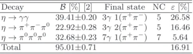
TABLE I. Characteristics of the η decay channels used to re-construct the ψ(3686) → γηπ+π−decays: branching fraction B, final state topology, number of constraints (NC) in the kinematic fit, and reconstruction efficiency, ε, according to exclusive phase-space MC.
Decay B[%] [2] Final state NC ε [%] η → γγ 39.41±0.20 3γ 1(π+π−) 5 26.58 η → π+π−π0 22.92±0.28 3γ 2(π+π−) 5 16.46 η → π0π0π0 32.68±0.23 7γ 1(π+π−) 7 5.64
A. χc1 →ηπ+π− event selection
The χc1 → ηπ+π− candidates in η three-pion decays
are selected by requiring that the invariant mass of three pions satisfy:
0.535 < m(3π) < 0.560 GeV/c2. (1) For the η → γγ candidates, we require that the mass constraint fit for η → γγ satisfies χ2
γγ < 15. The
χ2
N C obtained from four-momenta kinematic constraint
fits are required to satisfy χ2
5C < 40, χ25C < 40 and
χ2
7C < 56 for η → γγ, η → π+π −
π0 and η → 3π0,
respectively. These selection criteria effectively remove kaon and other charged track contamination, justifying the assumption that all charged tracks are pions. To select the χc1 candidates from the ψ(3686)→ γχc1
tran-sition, we require the energy of the radiative photon to satisfy 0.155 < Eγ< 0.185 GeV.
1. Background suppression
The major background for all final states comes from ψ(3686) → ηJ/ψ, while in the η → γγ case the back-ground from ψ(3686)→ γγJ/ψ decays is also significant. The background from ψ(3686) → ππJ/ψ is negligible, once a good η candidate is found.
To suppress ψ(3686)→ ηJ/ψ background for all three η decays, the system recoiling against the η, with respect to the ψ(3686), must have its invariant mass separated at least 20 MeV/c2from the J/ψ mass.
Additional selection criteria are used in the η → γγ channel to suppress π0 contamination and ψ(3686)
→ γγJ/ψ production. The former background is suppressed by rejecting events in which any two-photon combination satisfies 0.110 < m(γγ) < 0.155 GeV/c2. The latter
background is suppressed by vetoing events for which a two-photon combination not forming an η has a total energy between 0.52 GeV < Eγγ < 0.60 GeV. This range
of energies is associated with the doubly radiative decay ψ(3686)→ γχcJ; χcJ→ γJ/ψ, for which the energy sum
of two transitional photons is Eγγ≈ 0.560 GeV.
2. Background subtraction
The background estimated from the inclusive MC after all selection criteria are applied is below 3% in each chan-nel. The background from η sidebands is subtracted, and Fig. 1 shows the invariant mass distributions of η candi-dates with vertical dotted bars showing the η sideband regions. The sideband regions for the two-photon and three-pion modes are defined as 68 < |m(γγ) − mη| <
113 MeV/c2 and 37 <
|m(3π) − mη| < 62 MeV/c2,
re-spectively, where mη is the nominal η mass [2]. In the
case of η three-pion decays, the η signal region, defined by Eq. (1), is indicated by dash-dotted bars in Fig. 1. Although the mass distribution of three neutral pions, Fig. 1(c), is wider than the corresponding distribution from the charged channel, Fig. 1(b), we use the same selection criteria for both η decays, which keeps the ma-jority of good η→ 3π0 candidates and results in similar
background levels in the two channels. The effects of in-cluding more data from the tails of these distributions are taken into account in the systematic uncertainties. The invariant mass plot representing η→ γγ candidates, Fig. 1(a), is used only to select η sidebands for back-ground subtraction. Table I lists channel efficiencies and the effective efficiency for all channels.
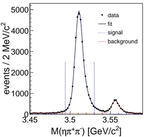
The ηπ+π− invariant mass distribution, when events
from all η channels are combined, is shown in Fig. 2. In the signal region, indicated by vertical bars, there are 33919 events, with the background of 497 events esti-mated from the η sidebands. The sideband background does not account for all the background, and after the η-sideband background is subtracted, the remaining back-ground is estimated by fitting the invariant mass distri-bution. The fit is shown by the solid distribution, Fig. 2. For the χc1 signal, a double-sided Crystal-Ball
distribu-tion (dotted) is used, and for the background, a linear function along with a Gaussian corresponding to the χc2
contribution (dashed) are used. The signal purity esti-mated from the fit isP = (98.5±0.3)%, where the error is obtained from fluctuations in the background when using different fitting ranges and shapes of the background.
B. Two-body structures in the χc1→ηπ+π− decays
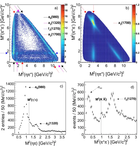
The Dalitz plot for selected signal events is shown in Fig. 3(a). Two-body structures reported in previous analyses of the χc1→ ηπ+π− decays, by BESII [26] and
CLEO [10, 27], the a0(980)π, a2(1320)π and f2(1270)η,
are indicated by the long-dotted, dashed and dash-dotted arrows pointing into the Dalitz space, respectively. One feature of this distribution is the excess of events in the upper left corner of the Dalitz plot (a), pointed to by the dotted arrows, which cannot be associated with known structures observed in previous analyses of this χc1 decay. We hypothesize this is due to a2(1700)
pro-duction. The expected Dalitz plot of a a2(1700)π signal is
shown in Fig. 3(b), obtained assuming that the a2(1700)
is the only structure produced. The a2(1700) → ηπ+
and a2(1700)→ ηπ− components cannot be easily
iden-tified along the dotted arrows in the Dalitz plot, Fig 3(a), but their crossing in the plot shown in Fig. 3(b) visually matches the excess of events in the upper left corner of the Dalitz plot of Fig. 3(a).
The distributions of the square of the invariant mass are shown in Fig. 3(c) for ηπ and (d) for π+π−
. Struc-tures that correspond to a0(980), a2(1320) and f2(1270)
] 2 ) [GeV/c γ γ M( 0.4 0.45 0.5 0.55 0.6 0.65 0.7 2 events / 2 MeV/c 0 500 1000 1500 2000 ] 2 ) [GeV/c γ γ M( 0.4 0.45 0.5 0.55 0.6 0.65 0.7 2 events / 2 MeV/c 0 500 1000 1500 2000 γ γ → η a) ] 2 ) [GeV/c 0 π -π + π M( 0.45 0.5 0.55 0.6 0.65 2 events / 2 MeV/c 0 500 1000 1500 2000 2500 ] 2 ) [GeV/c 0 π -π + π M( 0.45 0.5 0.55 0.6 0.65 2 events / 2 MeV/c 0 500 1000 1500 2000 2500 0 π -π + π → η b) ] 2 ) [GeV/c 0 π 0 π 0 π M( 0.45 0.5 0.55 0.6 0.65 2 events / 2 MeV/c 0 200 400 600 800 ] 2 ) [GeV/c 0 π 0 π 0 π M( 0.45 0.5 0.55 0.6 0.65 2 events / 2 MeV/c 0 200 400 600 800 0 π 0 π 0 π → η c)
FIG. 1. The invariant mass distribution of the η candidates, where dotted (red) lines indicate regions used for background subtraction, while dash-dotted bars (blue) show η-signal boundaries for the three-pion η decay cases. There are no blue bars on plot a) since the η → γγ signal is selected using the γγ kinematic constraint (color online).
production are evident, as well as a low-mass ππ peak, sometimes referred to as the σ state. In each of these two distributions there is a visible threshold effect. In the ππ distribution, there is a structure above the K ¯K threshold, which is too broad to result from the f0(980)
alone. In the ηπ distribution, the broadening of the a0(980) peak around 1.2 GeV2/c4 could be associated
with the η′
π threshold. By examining various regions in the Dalitz space, we conclude that the cross-channel con-tamination, or reflections, are not associated with these threshold effects in the data. In order to eliminate ground as the source of these peculiar line-shapes, back-ground studies are performed. Namely, we increased the background level by relaxing the kinematic constraint to χ2
N C/N C < 10 and also suppressed more background by
requiring χ2
N C/N C < 5. In addition we varied the limits
on tagging η and χc1candidates, as explained in Sec. V.
It is possible that the ππ line shape results from a destructive interference between the f0(980) and other
components of the ππ S-wave. It has been known for some time that the a0(980) → ηπ line shape is affected
by the proximity of the K ¯K threshold to the a0(980)
mass [28]. If the a0(980)→ η′π coupling appears to be
important for describing the a0(980)→ ηπ distribution,
this would be an example when a virtual channel is influ-encing the distribution of another decay channel, despite its threshold being far away from the resonance peak. We use an Amplitude Analysis (AA), described in the next section, to help in answering the above questions, and to determine the nature and significance of the “crossing structure” discussed.
III. AMPLITUDE ANALYSIS
To study the substructures observed in the χc1 →
ηπ+π− decays, we use the isobar model, in which it is
assumed that the decay proceeds through a sequence of two-body decays, χc1 → Rhb; R → h1h2, where either
an isospin-zero (R → ππ) or isospin-one (R → ηπ) res-onance is produced, with the total spin J, and relative
]
2) [GeV/c
-π
+π
η
M(
3.45 3.5 3.55 2events / 2 MeV/c
0 1000 2000 3000 4000 5000 data fit signal backgroundFIG. 2. Invariant mass of the χc1 candidates, after the η sideband background is subtracted. Vertical bars indicate the region used to select the χc1 candidates. See text for the fit discussion (color online).
orbital angular momentum L with respect to the bache-lor meson, hb. For resonances with J > 0, there are two
possible values of L that satisfy the quantum number conservation for the 1++
→ (JP C)0−
L transition.
We use the extended maximum likelihood technique to find a set of amplitudes and their production coefficients that best describe the data. The method and complete description of amplitudes constructed using the helicity formalism are given in Ref. [10], with two exceptions.
The first difference is that the events from the η−sidebands are subtracted in the likelihood function L, with equal weight given to the left-hand and right-hand sides, using a weighting factor ω = −0.5. The second difference with respect to Ref. [10] is that we deviate from the strict isobar model by allowing production am-plitudes to be complex. Isospin symmetry for ηπ±
reso-nances is imposed.
2
]
2) [GeV/c
+π
η
(
2M
0
2
4
6
8
10
2]
2) [GeV/c
-π
+π
(
2M
0
2
4
6
8
10
0 2 4 6 8 10 12 14 16 18 20a)
(980) 0 a (1320) 2 a (1700) 2 a (1270) 2 f 2]
2) [GeV/c
+π
η
(
2M
0
2
4
6
8
10
2]
2) [GeV/c
-π
+π
(
2M
0
2
4
6
8
10
0 0.2 0.4 0.6 0.8 1 1.2b)
(1700) 2 a 2]
2) [GeV/c
π
η
(
2M
0.5 1 1.5 2 2.5 3 3.5 2)
22 entries / 50 (MeV/c
0 200 400 600 800 1000 1200 1400 ) π ’ η ( 2 M (980) 0 a (1320) 2 a c) 2]
2) [GeV/c
-π
+π
(
2M
0 0.5 1 1.5 2 2.5 3 2)
2events / 50 (MeV/c
0 100 200 300 400 500 600 700 ) K (K 2 M π π σ (1270) 2 f d)FIG. 3. Dalitz plots obtained from selected χc1 candidates from (a) data and (b) exclusive MC, assuming the a2(1700) is the only structure produced. The (c) ηπ and (d) π+π−projections show various structures, which can also be identified by arrows in the Dalitz plot (a). Vertical dotted lines in plots (c) and (d) indicate the thresholds for producing the η′π or K ¯K in the ηπ or ππ space, respectively (color online).
In the minimization process of the expression−2 ln L, the total amplitude intensity, I(x), constructed from the coherent sum of relevant amplitudes, is bound to the number of observed χc1 candidates by using the integral
Nχc1 = Z
ξ(x)I(x)dx, (2)
where x represents the kinematic phase space, while ξ(x) is the acceptance function, with the value of one (zero) for accepted (rejected) exclusive MC events. The proper normalization of different η channels is ensured by using exclusive MC samples, generated with sample sizes pro-portional to the η branching fractions, listed in Table I. If the complete generated exclusive MC set is used in the MC integration, then Eq. (2) provides the acceptance
corrected number of χc1 events, adjusted by subtracted
background contributions. In this case, ξ(x)≡ 1 for all MC events. Fractional contributions, Fα, from specific
amplitudes, Aα, are obtained by restricting the coherent
sum in I(x) to Iα(x), so that
Fα=
R
Iα(x)dx
R
I(x)dx. (3)
The numerator represents acceptance-corrected yield of a given substructure, used to calculate relevant branching fractions, Bα. Errors are obtained from the covariance
matrix using proper error propagation, so for a given substructure, the errors onBαandFαare not necessarily
the same.
de-scribed by amplitudes constructed to take into account the spin alignment of the initial state and the helicity of the radiated photon. Linear combinations of helicity am-plitudes can be used to construct amam-plitudes in the mul-tipole basis, matching the electric dipole (E1) and mag-netic quadrupole (M 2) transitions. The ψ(3686)→ γχc1
decay is dominated by the E1 transition (CLEO) [29], and a small M 2 contribution (≈ 3%) can be treated as a systematic uncertainity.
A. Mass dependent terms, Tα(s)
The dependence of amplitude Aα on the energy can
be separated from its angular dependence, employing a general form pLqJT
α(s), if the width of the χc1 is
ne-glected. Here, p and q are decay momenta for decays χc1→ RJhb and RJ→ h1h2 in the rest frame of the χc1
and a resonance RJ, respectively, while s = m212 is the
squared invariant mass of the corresponding isobar prod-ucts (ππ or ηπ). For most resonances, we use relativistic Breit-Wigner (BW) distributions, with spin-dependent Blatt-Weisskopf factors [30]. For the a0(980) and ππ
S-wave line shapes, we use different prescriptions explained below.
To account for the non-resonant process χc1→ ηπ+π−,
we use an amplitude constructed as the sum of all pos-sible final state combinations of helicity amplitudes con-strained to have the same production strength, with no dependence on the invariant mass of the respective two-body combinations.
1. Parametrization of a0(980)
Instead of using the usual Flatt´e formula [28] to de-scribe the a0(980) line-shape, we use dispersion integrals,
following the prescription given in Ref. [20]. We consider three a0(980) decay channels, the ηπ, K ¯K, and η′π, with
corresponding coupling constants, gch, and use an
appro-priate dispersion relation to avoid the problem of a false singularity [31] present in the η′π mode (see discussion
at the end of this section). The a0(980) amplitude is
constructed using the following denominator: Dα(s) = m20− s −
X
ch
Πch(s), (4)
where m0is the a0(980) mass and Πch(s) in the sum over
channels is a complex function, with imaginary part ImΠch(s) = g2chρch(s)Fch(s), (5)
while real parts are given by principal value integrals
ReΠch(s) = 1 πP Z ∞ sch ImΠch(s′)ds′ (s′ − s) . (6)
In the above expressions ρch(s) is the available phase
space for a given channel, obtained from the correspond-ing decay momentum qch(s): ρch(s) = 2qch(s)/√s. The
integral in Eq. (6) is divergent when s→ ∞, so the phase space is modified by a form factor Fch(s) = e−βq
2
ch(s),
where the parameter β is related to the root-mean-square (RMS) size of an emitting source [20]. We use β = 2.0 [GeV/c2]−2 corresponding to RMS = 0.68 fm, and
we verify that our results are not sensitive to the value of β. The integration in Eq. (6) starts from the threshold for a particular channel, sch, which conveniently solves the
problem of the analytical continuation in special cases of final state configurations like the a0(980) → η′π, when
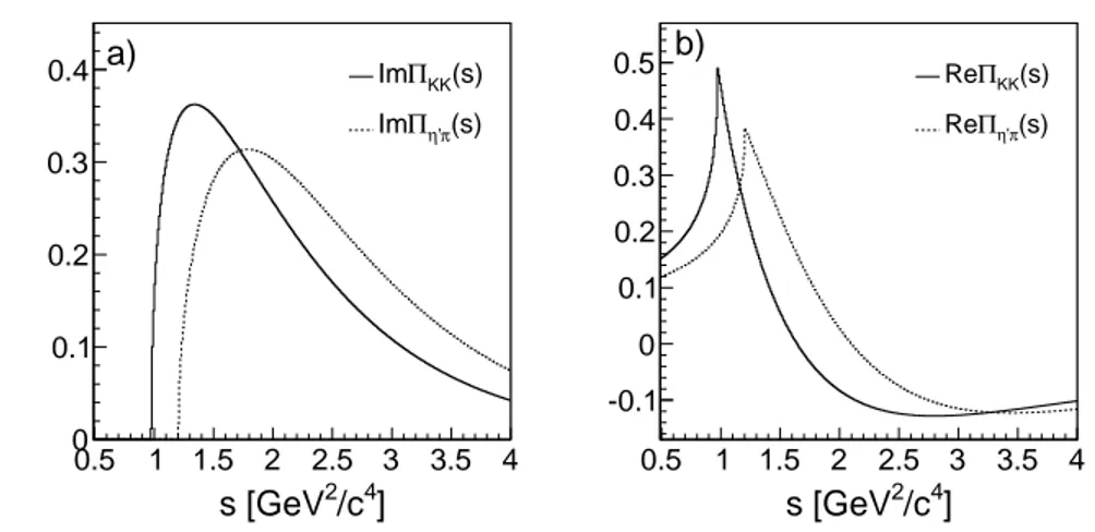
the decay momentum below the threshold (s < mη′+mπ) becomes real again for s < mη′− mπ. Figure 4 shows the
shapes of (a) ImΠch(s) and (b) ReΠch(s) (b), for the
K ¯K and η′
π channels, for arbitrary values of the cou-pling constants. In the final form, the real parts in the denominator of Eq. (4) are adjusted by ReΠch(m0) terms:
ReΠch(s)→ ReΠch(s)− ReΠch(m0).
2. ππ S-wave model
The ππ S-wave parametrization follows the prescrip-tion given in Ref. [10], in which two independent pro-cesses for producing a ππ pair are considered: direct (ππ)S → (ππ)S, and production through kaon loops,
(K ¯K)S → (ππ)S. Amplitudes corresponding to these
scattering processes, labeled Sππ(s) and SK ¯K(s), are
based on di-pion phases and intensities obtained from scattering data [32], which cover the ππ invariant mass region up to 2 GeV/c2. The S
ππ(s) component is adapted
in Ref. [10] to account for differences in the ππ production through scattering and decay processes, using the denom-inator, D(s), extracted from scattering experiments. The Sππ(s) amplitude in this analysis takes the form:
Sππ(s) = c0S0(s)+ X i=1 cizsiK ¯K(s)S 0(s)+X i=1 c′ izis′(s)S0(s). (7) The common term in the above expression, S0(s) = 1/D(s), is expanded using conformal transformations of the type zsth(s) = √s + s 0−√sth− s √s + s 0+√sth− s , (8)
which is a complex function for s > sth. Equation (7)
fea-tures two threshold-functions, zsth(s), one corresponds to
K ¯K production with sK ¯K = 4m2
K, while another with
sth= s′ could be used to examine other possible
thresh-old effects in di-pion production. The ci, i = 1, 2 are
production coefficients to be determined.
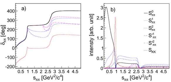
Figure 5 shows the (a) phase and (b) intensity of vari-ous components used in constructing the ππ S-wave am-plitude based on two functions given by Eq. (8), with
] 4 /c 2 s [GeV 0.5 1 1.5 2 2.5 3 3.5 4 0 0.1 0.2 0.3 0.4 ImΠKK(s) (s) π ’ η Π Im a) ] 4 /c 2 s [GeV 0.5 1 1.5 2 2.5 3 3.5 4 -0.1 0 0.1 0.2 0.3 0.4 0.5 (s) KK Π Re (s) π ’ η Π Re b)
FIG. 4. Line shapes of (a) ImΠ(s) and (b) ReΠ(s) for the K ¯K and η′π production with arbitrary normalization.
different thresholds: zK ¯K(s) and zs′(s). The follow-ing convention is used: Si
ππ(s) = zK ¯i KS
0(s), S′i ππ(s) =
zi
s′S0(s). Components are arbitrarily scaled, and we set
√ s′
∼ 1500 MeV/c2, similarly to the value used later in
analysis. The parameter s0= 1.5 (GeV/c2)2can be used
to adjust the left-hand cut in the complex plane, and the same value is used in all components.
IV. RESULTS
We present results from the amplitude analysis of the full decay ψ(3686)→ γχc1; χc1→ ηπ+π−, reconstructed
in three major η decay modes. The optimal solution to describe the data is found by using amplitudes with fractional contributions larger than 0.5% and significance larger than 5σ. The significance for each amplitude α is determined from the change in likelihood with respect to the null-hypothesis, ∆Λ = −2 ln L0/Lα. The
null-hypothesis for a given amplitude is found by excluding it from the base-line fit, and the corresponding amplitude significance is calculated taking into account the change in the number of degrees of freedom, which is two (four) for J = 0 (J > 0) amplitudes.
The most dominant amplitude in this reaction is a0(980)π, as evident from the ηπ projection of the Dalitz
plot, Fig. 3(c). Other amplitudes used in our base-line fit include the SK ¯Kη, Sππη, f2(1270)η, f4(2050)η,
a2(1320)π and a2(1700)π, where masses and widths of
resonances described by BW functions are taken from the PDG [2], while the a2(1700) and a0(980) parameters
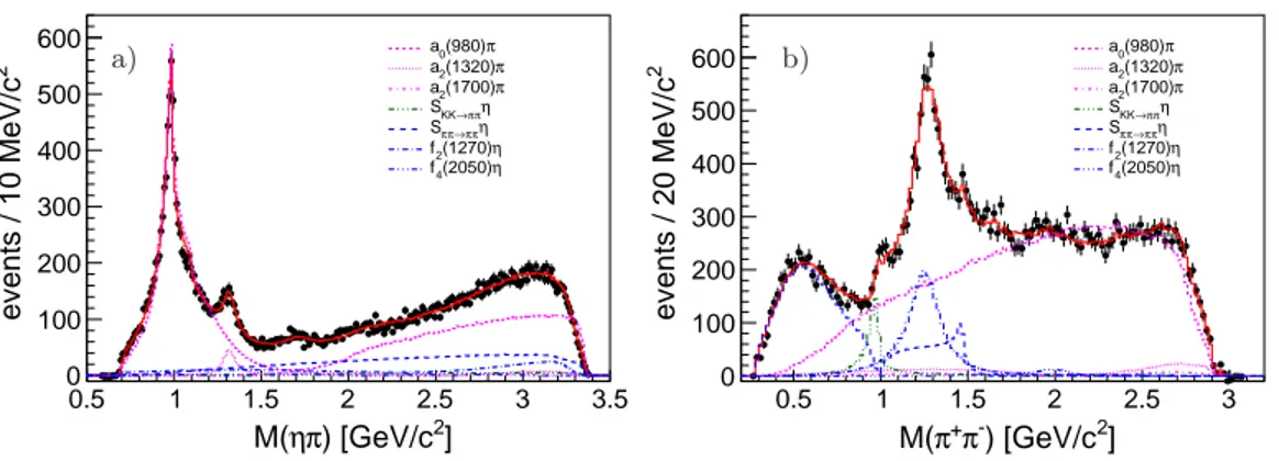
are free parameters to be determined by the fit in this work. The mass projections are shown in Fig. 6, and the corresponding fractional contributions and significances are listed in Table II. For amplitudes with spin J > 0 both orbital momentum components are included.
The following components form the Sππ(s) amplitude:
Sππ(s) = c0S0(s) + c1Sππ1 (s) + c ′
1Sππ′1(s) + c ′
2Sππ′2(s). (9)
As indicated earlier, the threshold used to construct the S1(s) term is s
K ¯K = 4m2K. The threshold for the S ′i(s)
components (i = 1, 2) is s′
= 2.23 [GeV/c2]2, which is
close to the mass of the f0(1500), and it is responsible
for the peaking of the Sππη amplitude in this region,
Fig. 6(b). In fact, the S′i(s) components are used instead
of the f0(1500)η amplitude, which would be needed in the
optimal solution if only threshold functions zi
K ¯K(s) were
used in the expansion of the Sππ(s)η amplitude. With
these additional terms, the contribution and significance of ππ scalars, the f0(1370), f0(1500) and f0(1710), is
negligible, for each. Although this particular set of am-plitudes respects the unitarity of the ππ S-wave, we use the sum of BW to model other spins and final states, namely the f2(1270), f4(2050), a2(1320) and a2(1700).
Our approach provides reasonable modeling of the ππ line shape, and the sum of all ππ S-wave components, SK ¯K and Sππ, is reported in Table II.
Besides the f0(1370), f0(1500), and f0(1710), other
conventional resonances are probed, including the f0(1950), f2(1525), f2(2010), and a0(1450), with
param-eters fixed to PDG values [2]. They do not pass the tests for significance and fractional contribution. The non-resonant χc1 → ηπ+π− production is found to be
negligible. The search for possible 1−+resonances in the
ηπ final state will be presented below.
A. The a2(1700) signature
All structures listed in Table II have been already re-ported in the decay χc1→ ηπ+π−, except the a2(1700)π.
Its fractional contribution is around 1%, and the signifi-cance of each orbital momentum component is more than 10σ. Detailed background studies are performed to en-sure that the background, remaining after η-sideband subtraction, is not affecting the significance and frac-tional contribution of the a2(1700). Results of fitting
]
4/c
2[GeV
π πs
0.5 1 1.5 2 2.5 3 3.5 4 4.5[deg]
ππδ
-200 -100 0 100 200 300 400a)
]
4/c
2[GeV
π πs
0.5 1 1.5 2 2.5 3 3.5 4 4.5intensty [arb. unit]
0 0.5 1 1.5 2 2.5 3 π π 0
S
π π 1S
π π 2S
π π 1S’
π π 2S’
KKS
b)
FIG. 5. The (a) phase and (b) intensity of the ππ S-wave components. Red (dash) histograms represent the SK ¯K amplitude, blue histograms (dot and dash-dot) are obtained using Si
ππ = ziK ¯KS
0
ππ terms, while purple (long-dash-dot and dash-three-dot) represent Sππ′i = zsi′Sππ0 terms (color online).
TABLE II. Fractional intensities F, and significances of amplitudes in the base-line fit, with the first and second errors being statistical and systematic, respectively. The third error for the branching fractions for the χc1→ηπ+π−decay and decays into significant conventional isobars is external (see text). For exotic mesons only statistical errors on their fractional contributions are provided. The upper limits for exotic meson candidates, which include both statistical and systematic uncertainties, are at the 90% confidence-level. The coherent sum of all ππ S-wave components, (π+π−)
Sη, is included in this report. Note, the branching fractions for amplitudes of the type Aαη, involving isobars decaying into π+π−, are the products of χc1→Aαη and Aα→π+π−rates. Branching fractions for isobars decaying into ηπ include charge conjugates.
Decay F [%] Significance [σ] B(χc1→ηπ+π−) [10−3] ηπ+π− - - 4.67 ± 0.03 ± 0.23 ± 0.16 a0(980)+π− 72.8 ± 0.6 ± 2.3 > 100 3.40 ± 0.03 ± 0.19 ± 0.11 a2(1320)+π− 3.8 ± 0.2 ± 0.3 32 0.18 ± 0.01 ± 0.02 ± 0.01 a2(1700)+π− 1.0 ± 0.1 ± 0.1 20 0.047 ± 0.004 ± 0.006 ± 0.002 SK ¯Kη 2.5 ± 0.2 ± 0.3 22 0.119 ± 0.007 ± 0.015 ± 0.004 Sππη 16.4 ± 0.5 ± 0.7 > 100 0.76 ± 0.02 ± 0.05 ± 0.03 (π+π−) Sη 17.8 ± 0.5 ± 0.6 - 0.83 ± 0.02 ± 0.05 ± 0.03 f2(1270)η 7.8 ± 0.3 ± 1.1 > 100 0.36 ± 0.01 ± 0.06 ± 0.01 f4(2050)η 0.6 ± 0.1 ± 0.2 9.8 0.026 ± 0.004 ± 0.008 ± 0.001
Exotic candidates U.L. [90% C.L.]
π1(1400)+π− 0.58±0.20 3.5 < 0.046
π1(1600)+π− 0.11±0.10 1.3 < 0.015
π1(2015)+π− 0.06±0.03 2.6 < 0.008
are consistent with the values listed by the PDG [2]. To check how the a2(1700) parameters and fractional
con-tributions are affected by the f2(1270) and a2(1320), we
also fitted their masses and widths, which are provided in Table III with statistical uncertainties only. The mass (width) of the f2(1270) is lower (higher) than its nominal
value [2], maybe because of interference with underlying ππ S-wave components or threshold effects, other than those for the K ¯K or f0(1500) production.
The systematic uncertainties for the a2(1700) mass and
width are obtained by varying parameters of other am-plitudes within respective uncertainties listed in Ref. [2], and taking into account variations listed in Table III.
The a0(980) errors are shown in Table IV. Variations
in the shape of the ππ-S wave amplitude are taken into account by changing terms in the expansion, Eq. (9).
We also test the significance of the a2(1700)
includ-ing alternative states with the same mass and width, but different spins: J = 0, 1, 4. In all cases, the significance of the a2(1700) in the presence of an alternative state
exceeds 17σ. The statistical significance of the a2(1700)
signal alone is 20σ. This result confirms our hypothesis based on a visual inspection of the Dalitz plot, Fig. 3(a), that the excess of events in the upper left corner of the Dalitz space results from the a2(1700) production, and
] 2 ) [GeV/c π η M( 0.5 1 1.5 2 2.5 3 3.5 2 events / 10 MeV/c 0 100 200 300 400 500 600 a0(980)π π (1320) 2 a π (1700) 2 a η π π → KK S η π π → π π S η (1270) 2 f η (2050) 4 f a) ] 2 ) [GeV/c -π + π M( 0.5 1 1.5 2 2.5 3 2 events / 20 MeV/c 0 100 200 300 400 500 600 a0(980)π π (1320) 2 a π (1700) 2 a η π π → KK S η π π → π π S η (1270) 2 f η (2050) 4 f b)
FIG. 6. Projections in the (a) ηπ and (b) π+π−invariant mass from data, compared with our base-line fit (solid curve) and corresponding amplitudes (various dashed and dotted lines). All features of the data, including structures discussed in Sec. II B are reproduced rather well.
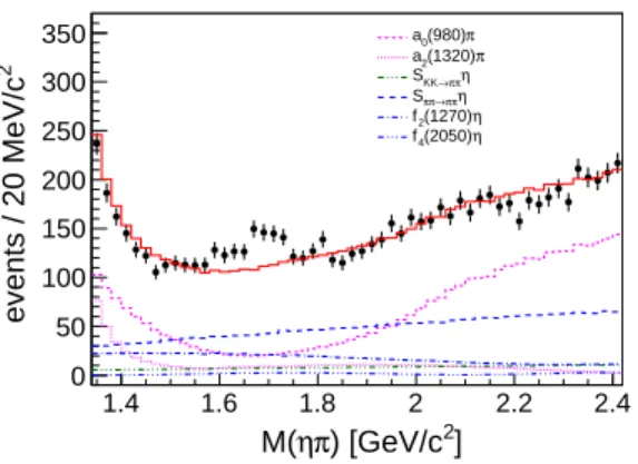
and a2(1700)−π+components. Further, Fig. 7 shows the
ηπ mass distribution in the region around the expected a2(1700) peak, where data points are compared with a
fit when the a2(1700)π amplitude is excluded.
B. a0(980) parameters
When determining the a0(980) parameters we use the
ratios R21= g2K ¯K/g2ηπ, and R31= g2η′π/gηπ2 . The
result-ing values are listed in Table IV, where systematic uncer-tainties are obtained by fitting the a0(980) parameters
under different conditions. The level of background is varied by changing selection criteria described in Sec. II, and by changing the amount of background subtracted from the η sidebands. Effects of the line shapes of the a2(1320), a2(1700), f2(1270) and f4(2050) resonances are
taken into account by varying their masses and widths within the respective uncertainties [2], and using values from Table III. The effect of the ππ S-wave shape is examined in similar way as for the a2(1700). The
pres-ence of alternative conventional and exotic resonances is also taken into account. Our result is not sensitive to the value of the parameter β in Eqs. (5) and (6), within the range of values: β = (2.0± 1.0) [GeV/c2]2.
For comparison we list two previous results, one from a similar experiment, CLEO-c, and the other obtained using Crystal Barrel data. There is a general agreement between different analyses for the a0(980) mass and R21.
The ratio R31 was fixed in Ref. [20] to the theoretical
value provided by Eq.(11), while it was consistent with zero in the CLEO-c analysis, possibly because of smaller statistics. It is not easy to comment on the difference in values for the ηπ coupling, which could be affected by different normalizations used by different analyses.
This analysis provides the first non-zero measurement of the coupling constant gη′π. To test the sensitivity of the a0(980)→ ηπ line shape to the decay a0(980)→ η′π,
we repeat the analysis with gη′π = 0, and let the values of the other parameters free. The results of this fit are also given in Table IV. The likelihood change when the η′
π channel is ignored shows that the significance of a non-zero gη′π measurement is 8.9σ. The same result is obtained when the analysis is performed in the presence of the a0(1450). The values of the two ratios based on
the SU(3) expectation are
gK ¯2K/gηπ2 = 1/(2 cos2φ) = 0.886± 0.034, (10) gη2′π/g 2 ηπ = tan 2φ = 0.772 ± 0.068, (11) which depend on the choice of the η−η′
mixing angle; φ = (41.3±1.2)◦
in this case [20]. Our result is consistent with Eq. (11) within 1.5σ, based on the quoted uncertainties.
C. Search for ηπ P -wave states
We examine possible exotic meson production in the ηπ invariant mass region from 1.4 to 2.0 GeV/c2.
Ta-ble II lists fractional contributions and significances of three JP C = 1−+ candidates, added one at the time to
our nominal fit. Two possible orbital-momentum config-urations for an exotic amplitude are the S-wave and D-wave, and the significance of each is tested individually. We find that the significance of the S-wave is marginal, less than 2σ for every π1, and the reported significances
in Table II result from using the S and D waves together in the fit. The most significant of the three possible ex-otic states is the π1(1400), with a significance of 3.5σ and
fractional contribution less than 0.6%. This represents a weak evidence for the existence of the π1(1400) because
in alternative amplitude configurations, when parame-ters of other amplitudes are varied, the significance of this state becomes < 3σ. In the nominal amplitude con-figuration, the significance of each π1(1400) component is
] 2 ) [GeV/c π η M( 1.4 1.6 1.8 2 2.2 2.4 2 events / 20 MeV/c 0 50 100 150 200 250 300 350 a0(980)π π (1320) 2 a η π π → KK S η π π → π π S η (1270) 2 f η (2050) 4 f
FIG. 7. The ηπ invariant mass projection from data in the region (1.3, 2.4) GeV/c2, compared with the fit without the a2(1700)η amplitude (solid curve). Other amplitudes are plotted (various dashed and dotted lines) for comparison, while the peak that is associated with the a2(1700) is evident.
TABLE III. The mass and width of the a2(1700), with statistical and systematic uncertainties. Only statistical uncertainties from the f2(1270) and a2(1320) fits are listed. Comparison with the PDG [2] values is provided, with all units in GeV/c2.
BESIII PDG [2]
Resonance M Γ M Γ
a2(1700) 1.726±0.012±0.025 0.190±0.018±0.030 1.732±0.016 0.194±0.040 f2(1270) 1.258±0.003 0.206±0.008 1.275±0.001 0.185±0.003 a2(1320) 1.317±0.002 0.090±0.005 1.318±0.001 0.107±0.005
of the S-wave is much smaller than the D-wave contri-bution, pointing that the evidence for the π1(1400) is
circumstantial.
Masses and widths of the three exotic candidates are not very well constrained by previous analyses, and we vary the respective parameters within listed limits [2]. Our conclusion is that there is no significant evidence for an exotic ηπ structure in the χc1→ ηπ+π− decays, and
we determine upper limits at the 90% confidence level for the production of each π1 candidate.
D. Branching fractions
The branching fraction for the χc1→ ηπ+π− decay is
given by
B(χc1→ ηπ+π−) = P ∗ Nχc1
→ηπ+π− Nψ(3686)Bψ(3686)→γχc1Bηǫ
, (12)
where the branching fractions Bψ(3686)→γχc1 and Bη are from Ref. [2]; the latter is listed in Table I. The num-ber of ψ(3686), Nψ(3686), [23, 24] is provided in Sec II.
The signal purity, P, given in Sec. II A 1, takes into ac-count that the number of χc1 obtained from the
ampli-tude analysis includes the background not accounted for by the sideband subtraction. Using Eq. (2) we obtain
Nχc1 = 192658± 1075, where the error is from the co-variance matrix. The efficiency in Eq. (12) is ǫ≡ 1, by construction.
Table II lists the branching fraction for the χc1 →
ηπ+π−
, and branching fractions for subsequent reso-nance production in respective isospin states, ηπ±
or π+π−
, where the first and second errors are statistical and systematic, respectively. The branching fraction for a given substructure is effectively a product:
Bα=Fα× B(χc1→ ηπ+π−), (13)
obtained using generated exclusive MC in accordance with Eq. (3). The third error is external, associated with uncertainties in the branching fractions for the radiative transition ψ(3686)→ γχc1 and η decays. We also show
the total π+π−
S-wave contribution, obtained from the coherent sum of the SK ¯K and Sππ components.
Statis-tical errors, as well as systematic ones, for a given frac-tional contribution and branching fraction differ, because common systematic uncertainties for all amplitudes can-cel when fractions are calculated, which will be discussed below.
The upper limits for the production of the π1(1400)π,
π1(1600)π, and π1(2015)π are shown in Table II. The
limits are determined by including the corresponding am-plitude in the nominal fit, one at a time. The analysis is repeated by changing other amplitude line shapes, and the background level, in a similar fashion used for
deter-TABLE IV. Parameters of the a0(980) determined from the fit using the dispersion relation of Eqs. (4-6), compared to results from previous analyses. Bold values indicate quantities that are fixed in the fit.
Data m0 [GeV/c2] gηπ2 [GeV/c2]2 g2K ¯K/g 2 ηπ gη2′π/gηπ2 CLEO-c [10] 0.998 ± 0.016 0.36 ± 0.04 0.872 ± 0.148 0.00 ± 0.17 C.Barrel [20] 0.987 ± 0.004 0.164 ± 0.011 1.05 ± 0.09 0.772 BESIII 0.996±0.002±0.007 0.368±0.003±0.013 0.931±0.028±0.090 0.489±0.046±0.103 BESIII (R2 31≡0) 0.990±0.001 0.341±0.004 0.892±0.022 0.0
mining systematic uncertainties of nominal amplitudes (see Sec. V). Masses and widths of exotic candidates are also varied within limits provided by the PDG [2]. The largest positive deviation of the exotic candidate yield with respect to the corresponding yield from the mod-ified nominal fit is effectively treated as the systematic error, summed in quadrature with the statistical error on a given exotic state yield. The resulting uncertainty is used to determine the 90% confidence level deviation, and added to the ’nominal’ yield of an exotic candidate to obtain the corresponding upper limit for the branching fraction B(χc1→ π1+π
−
).
The branching fractions for the substructures in χc1→
ηπ+π−
decays reported by the PDG [2] are compared in Table V with the values measured in this work, and with the previous most precise measurement (CLEO-c) [10]. The measurement for the f2(1270) production is adjusted
to account for the measured relative f2(1270)→ π+π−
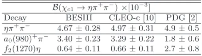
width. There is a rather large discrepancy between the values for the two most dominant substructures listed by the PDG and the two most recent measurements. There is very good agreement between the last two mea-surements, suggesting that the PDG values on two-body structures observed in χc1→ ηπ+π−need to be updated.
TABLE V. Comparison between recent measurements of the branching fractions B(χc1 → ηπ+π−), and with the PDG values.
B(χc1→ηπ+π−) ×[10−3]
Decay BESIII CLEO-c [10] PDG [2] ηπ+π− 4.67 ± 0.28 4.97 ± 0.31 4.9 ± 0.5 a0(980)+π− 3.40 ± 0.23 3.29 ± 0.22 1.8 ± 0.6 f2(1270)η 0.64 ± 0.11 0.66 ± 0.11 2.7 ± 0.8
V. SYSTEMATIC UNCERTAINTIES
Tables VI summarizes various contributions to the sys-tematic uncertainties in determining the χc1 → ηπ+π−
branching fraction, and Table VII shows the systemat-ics on the fractional contributions of amplitudes in the nominal fit. Systematic uncertainties in determining the
χc1 → ηπ+π− branching fraction stem from
uncertain-ties in charged track and shower reconstruction efficien-cies, the contribution of the M 2 multipole transition, amplitude modeling, the background contribution, and the uncertainty in the number of ψ(3686) produced at BESIII [23, 24]. External sources of uncertainty include the branching fraction B(ψ(3686)→ γχc1) and the
frac-tion of η decays, B(η) in Eq. (12). The external error affects only branching fractions, not fractional contribu-tions, and it is reported as a separate uncertainty.
Systematic uncertainties associated with the tracking efficiency and shower reconstruction are 1% per track and 1% per photon. Because of different final states used in this analysis, tracking and photon uncertainties are weighted according to the product of branching fractions and efficiencies of the different η channels, as listed in Ta-ble I. The resulting systematic uncertainties for charged tracks and photons are 2.47% and 3.92%, respectively.
The electromagnetic transition ψ(3686) → γχc1 is
dominated by the E1 multipole amplitude with a small fraction of the M 2 transition [29]. The nominal fit takes only the E1 multipole amplitude. Adding a small con-tribution of the M 2 helicity amplitude, of 2.9%, we find a difference in the branching fraction of 0.62%. This is taken as a systematic uncertainty.
When considering the effects of modeling line-shapes of different amplitudes, we repeat the analysis changing the mass and width of resonances, a2(1320), f2(1270),
and f4(2050), within respective uncertainties, and change
the a0(980) and a2(1700) parameters within the
lim-its of their statistical uncertainties, given in Tables IV and III. We also change BW line shapes by replacing spin-dependent widths with fixed widths, and take into account the χc1width and centrifugal barrier as another
systematic error. The largest effect from all these sources is taken as a systematic uncertainty for the branching fractions and fractional contributions.
The effect of background is estimated by varying the kinematic-constraint requirement, changing limits on tagging η and χc1candidates, changing the level of
sup-pression of the J/ψ and π0 productions, and the level
of background subtraction. As a general rule, selection criteria were changed to allow for≈ 1σ additional back-ground events, based on the numbers from the inclusive MC. We use χ2
varying the kinematic constraint. Based on these vari-ations, we conclude that the systematic uncertainty as-sociated with the assumption that all charged tracks are pions is negligible. To select χc1 candidates, we use
pho-ton energy ranges of (0.152-0.187) GeV, in the η → γγ channel, and (0.150-0.190) GeV, in two η → 3π chan-nels. The mass window for the η selection is changed to (0.530-0.565) GeV/c2. The π0suppression window is
re-duced to (0.120-0.150) GeV/c2and the J/ψ suppression
is reduced by vetoing two-photon energy within (0.525-0.595) GeV. We also determine the branching fractions without background subtraction from η-sidebands, and the largest effect is listed in Tables VI and VII.
Some uncertainties that are common for all ampli-tudes, like tracking, shower reconstruction, and Nψ(3686)
errors, cancel out in the fractional contributions. How-ever, they are taken into account when branching frac-tions are determined.
TABLE VI. Systematic uncertainties in determining the branching fraction B(χc1 → ηπ+π−). The systematic un-certainty per track is 1.0%, and for photons it is 1.0% per shower.
Contribution Relative uncertainty (%)
MDC tracking 2.5 photon detection 3.9 M 2/E1 0.6 Background 1.6 Amplitude modeling 0.1 Nψ(3686) 0.7 Total 5.0 External 3.4
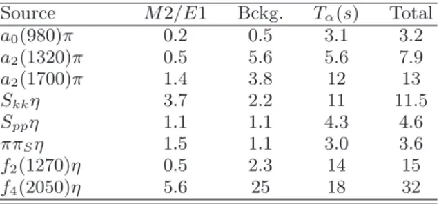
TABLE VII. Systematic uncertainties in fractional contribu-tions, in percent, for the base-line amplitudes used to model the χc1 →ηπ+π− decays.
Source M 2/E1 Bckg. Tα(s) Total
a0(980)π 0.2 0.5 3.1 3.2 a2(1320)π 0.5 5.6 5.6 7.9 a2(1700)π 1.4 3.8 12 13 Skkη 3.7 2.2 11 11.5 Sppη 1.1 1.1 4.3 4.6 ππSη 1.5 1.1 3.0 3.6 f2(1270)η 0.5 2.3 14 15 f4(2050)η 5.6 25 18 32 VI. SUMMARY
We analyze the world’s largest χc1→ ηπ+π− sample,
selected with very high purity, and find a very promi-nent a0(980) peak in the ηπ±invariant mass distribution.
An amplitude analysis of the ψ(3686) → γχc1; χc1 →
ηπ+π−
decay is performed, and the parameters of the a0(980) are determined using a dispersion relation. The
a0(980) line shape in its ηπ final state appears to be
sen-sitive to the details of the a0(980)→ η′π production, and
for the first time, a significant non-zero coupling of the a0(980) to the η′π mode is measured with a statistical
significance of 8.9σ.
We also report a2(1700)π production in the χc1 →
ηπ+π−
decays for the first time, with the mass and width in agreement with world average values, and this analy-sis provides both qualitative and quantitative evidence for the existence of the a2(1700). First, the signature of
the a2(1700) in the Dalitz space is consistent with the
ob-served Dalitz plot distribution. Second, the a2(1700)
sig-nificance from the amplitude analysis is larger than 17σ, compared to alternative spin assignments, even though the fractional yield of the a2(1700)π is only 1%. This
may help in listing the a2(1700) as an established
reso-nance by the the PDG [2].
We examine the production of exotic mesons that might be expected in the χc1 → ηππ decays: the
π1(1400), π1(1600) and π1(2015). There is only weak
evidence for the π1(1400) while other exotic candidates
are not significant, and we determine the upper limits on the respective branching fractions.
ACKNOWLEDGMENTS
The BESIII collaboration thanks the staff of BEPCII and the IHEP computing center for their strong sup-port. This work is supported in part by National Key Basic Research Program of China under Contract No. 2015CB856700; National Natural Science Founda-tion of China (NSFC) under Contracts Nos. 11235011, 11322544, 11335008, 11425524; the Chinese Academy of Sciences (CAS) Large-Scale Scientific Facility Pro-gram; the CAS Center for Excellence in Particle Physics (CCEPP); the Collaborative Innovation Center for Par-ticles and Interactions (CICPI); Joint Large-Scale Scien-tific Facility Funds of the NSFC and CAS under Con-tracts Nos. U1232201, U1332201; CAS under Con-tracts Nos. KJCX2-YW-N29, KJCX2-YW-N45; 100 Talents Program of CAS; National 1000 Talents Pro-gram of China; INPAC and Shanghai Key Laboratory for Particle Physics and Cosmology; Istituto Nazionale di Sic Nucleare, Italy; Joint Large-Scale Scientific Fa-cility Funds of the NSFC and CAS under Contract No. U1532257; Joint Large-Scale Scientific Facility Funds of the NSFC and CAS under Contract No. U1532258; Koninklijke Nederlandse Akademie van Wetenschap-pen (KNAW) under Contract No. 530-4CDP03; Min-istry of Development of Turkey under Contract No. DPT2006K-120470; The Swedish Resarch Council; U. S. Department of Energy under Contracts Nos. DE-FG02-05ER41374, DE-SC-0010504, DE-SC0012069; U.S.