WELFARE EFFECTS OF COASEAN TRANSACTIONS:
A GENERALIZED GRAPHICAL APPROACH
A. Bora OCAKCIOĞLU, Ph. D. Professor Ronald Coase published only a few articles during his career, but
he was awarded the Nobel Prize. This tells us that what counts in scientific publication is contribution not multiplicity.
Abstract
This article is about the graphical description and analysis of the welfare ef-fects of the Coasean1 transactions between the polluters and the pollutees.2 Pro-fessor Coase, in an article entitled The Problem of Social Cost (1960)3 asserted that in the absence of transaction costs, the opposed parties involved in an activity having “harmful effects” on each other may reach within the market an agree-ment that can lead to an efficient allocation regardless of the initial endowagree-ment of the property rights. According to this agreement, when the polluter has the prop-erty right (the right to pollute) the pollutee will offer him/her an indemnity to cease or decrease the activity causing the pollution. On the contrary, when the pollutee has the property right (the right not to be polluted) this time the polluter will offer him/her an indemnity to buy the right to pollute. Ronald Coase put the problem as the following: “This paper is concerned with those actions of business firms which have harmful effects on others…The economic analysis of such a sit-uation has usually proceeded in terms of divergence between the private and so-cial product of the factory in which economists have largely followed the treat-ment of Pigou in The Economics of Welfare.”4 As we know, Professor Pigou in his book “Economics of Welfare” proposed that the government can correct the dis-torted market allocation caused by externalities by imposing an appropriate tax on the polluter. This is what today is called the Pigouvian5 tax. The Pigouvian tax is imposed on the polluter as the price of polluting with a view to decrease it (ac-tually this approach is taught even today in modern books of public finance.) But Coase asserts that approaching the problem via Pigouvian taxes is of reciprocal nature: because, Pigouvian taxes designed to eliminate the harm on the pollutee inflict harm on the polluter. As a matter of fact a Pigouvian tax decreases produc-tion and consequently part of the producer’s surplus (and also the consumer sur-plus of the concerning consumers.) According to Coase instead of Pigouvian taxes the conflicting parties may reach an agreement within the market framework in which the party who does not have the property right may offer an indemnity to the other party having it. George Stigler called Coase’s argument as “theorem”6. After Coase a large number of scholars went over the matter. An immense
Professor of Economics and Public Finance, The School of Applied Sciences, Kadir Has University, Istanbul.
ture was developed on the subject. Some of the articles were against and some for the Coase’s assertion. Here in this article none of these are discussed and the va-lidity of the Coasean assumptions and propositions are not questioned at all. The original contributions in this article are the following: 1-The generalization of the cases or models within which the polluters and the pollutees can bargain; 2-The microeconomic equilibrium of the concerning parties after the transaction; 3- The welfare change of each side after the transaction. This article takes the Coase’s assertion as valid and uses the tools of the public sector economics and especially of cost-benefit analysis in the description of different possible transaction cases and equilibrium analyses.
Key Words: Coase Theorem; Pigouvian Tax; Property Right; Invariable
Technology; Variable Technology; Marginal Pollution Damage Cost; Marginal Utility Function of the Pollutee; Marginal Cleaning Cost; Consumer’s Surplus; Producer’s Surplus; Indemnity Supply Curve.
Coasevarî Ġşlemlerin Refah Etkileri: Genelleştirilmiş Grafiksel Bir Yaklaşım Profesör Ronald Coase akademik yaşamında az sayıda makale yayınlamış,
buna karşın kendisine Nobel Ödülü verilmiştir. Bu bize bilimsel yayınlar konusunda sayının değil katkının önemli olduğunu göstermektedir.
Özet
Bu makale kirletenlerle kirlenenler arasındaki Coasevarî1
işlemlerin refah etkilerinin grafiksel betimlenmesi ve analizi hakkındadır.2 Profesör Coase, Sosyal Maliyet (1960) başlıklı bir makalesinde, işlem maliyetlerinin olmadığı bir durum-da ve kişilerin birbirine yönelik “zararlı etkilerinin” bulunduğu bir faaliyette, hasım olan tarafların ilk mülkiyet haklarının dağılımına bakılmaksızın piyasa çerçevesinde etkin kaynak dağılımı sağlayan bir anlaşmaya varabileceklerini ileri sürmüştür. Bu anlaşmaya göre mülkiyet hakkı (kirletme hakkı) kirleten kişiye ait olduğu zaman kirlenen kişi kirletene, kirlenmeye sebep olan faaliyetin durdurulması veya azaltılması için bir tazminat ödeyecektir. Aksine, kirlenen kişi mülkiyet hakkına sahip ise bu kez kirleten kişi diğerine kirletme hakkını satın al-mak üzere bir tazminat vermeyi önerecektir. Ronald Coase problemi şu şekilde ifade etmektedir: “Bu makale başkalarına yönelik zararlı etkileri olan işletmelerin faaliyetleri ile ilgilidir. Böyle bir durumun ekonomik analizi genellikle iktisatçıların geniş ölçüde Pigou’nun Refah Ekonomisindeki yaklaşımını takip et-tikleri, fabrikanın özel ve sosyal ürünü arasındaki ayrışıma ilişkin olarak yapılagelmiştir.”3
Bildiğimiz gibi Profesör Pigou “Refah Ekonomisi” adlı kitabında devletin, dışsallıkların mevcudiyeti ile bozulmuş olan piyasa kaynak dağılımını, kirletene uygun bir vergi salmak sureti ile düzeltebileceği önerisinde bulunmuştur. Bu bugün Pigouvarî vergi olarak anılan vergidir. Pigouvarî vergi kirliliği gidermek için kirletene kirletmenin bedeli olarak salınır (aslında bu yaklaşım günümüzde dahi modern kamu maliyesi kitaplarında öğretilmektedir). Ancak Coase probleme Pigouvarî vergilerle yaklaşımda mütekabiliyet bulunduğunu ileri sürmüştür: çünkü, kirlenene yönelik zararlarının giderilmesini sağlamak için tasarlanan Pigouvarî vergiler kirletene de zarar vermektedir. Gerçekte Pigouvarî bir vergi üretimi ve buna bağlı olarak üretici fazlasının bir kısmını (ve ilgili tüketicilerin tüketici fazlasını da) azaltır. Coase’a göre Pigouvarî
vergilerin uygulanması yerine, hasım taraflar piyasa çerçevesi içinde mülkiyet hakkına sahip olmayan tarafın diğerine tazminat verdiği bir anlaşmaya varabilir-ler. George Stigler Coase’ın iddiasına “Coase Teoremi” adını vermiştir6. Coase’dan sonra çok sayıda bilim adamı bu konu üzerine gitmişlerdir. Bu konuda büyük bir literatür oluşmuştur. Bu konuda yazılan makalelerden bazıları Coase’un iddiasının aleyhine diğer bazıları lehine tavır almışlardır. Bu makalede söz konusu makalelerin hiçbiri tartışılmamakta ve Coasevarî varsayımlar ve öne-riler sorgulanmamaktadır. Bu makaledeki original katkılar şunlardır: 1- Kirleten-lerin ve kirlenenKirleten-lerin pazarlık yapacakları vakaların ve modelKirleten-lerin genelleştirilmesi; 2- Anlaşmadan sonra ilgili tarafların mikroekonomik dengeleri; 3-İşlemden sonra her bir tarafın refahındaki değişme. Bu makale Coase’un iddiasını geçerli olarak kabul etmekte ve farklı işlem vakalarının betimlenmesinde ve denge analizlerinde kamu kesimi ekonomisi ve özellikle maliyet-fayda analizi araçlarını kullanmaktadır.
Anahtar Kelimeler: Coase Teoremi; Pigouvarî Vergi; Mülkiyet Hakkı;
Değişmez Teknoloji; Değişken Teknoloji; Marjinal Kirletme Zarar Maliyeti; Kir-lenenin Marjinal Yarar Fonksiyonu; Marjinal Temizleme Maliyeti; Tüketici Fazlası; Üretici Fazlası; Tazminat Arz Eğrisi.
1. Concepts, Tools and Assumptions. The method used in this article consists of using concepts, assumptions and analyses familiar in public sector economics. Here are some of these:
Consumer Surplus; Producer’s Surplus; Normal Profit; Economic Profit: The consumer’s and producer’s surpluses are monetized measures of welfare. Any change in consumer’s and producer’s surplus reflects an equal change in welfare. The normal profit is the long-run equilibrium profit or the opportunity cost of doing business of the perfectly competitive firm. Any profit above nor-mal profit is the economic profit which can only be realized in the short-run.
The assumption that the perfect competition firm’s supply function also includes the “normal profit” (as part of marginal cost) distorts this article’s ap-proach, therefore here in this article it is assumed that the supply curve of the firm (the marginal cost curve) did not include the normal profit; Following this, the difference (as area) between the revenue curve (the flat demand curve di-rected to the perfectly competitive firm) and the firm’s supply curve becomes equal not only to the economic profit but also to economic profit plus normal profit (in other words total revenue minus total cost which is the integral of the marginal cost function.) This difference is also the producer’s surplus (fig. 3). So, in this article the producer’s surplus is equal to the economic profit plus normal profit.
The Marginal Pollution Damage Cost Function and the Marginal Utility Function of the Pollutee: The pollution damage cost (monetized pollution dam-age) inflicted by the polluter on the pollutee is represented by the marginal pol-lution damage cost function (KL in Fig. 1). The marginal polpol-lution damage cost function is presumably an increasing one. In the rightward direction to the ori-gin O the marori-ginal pollution damage cost function is an increasing external marginal cost function. But in the opposite direction and to the origin O’ (We have two superposed axes systems and two origins O and O’ in all the graphs) the same curve (LK in Fig. 1) is a marginal utility function again for the pollu-tee B; because, any reduction of the pollution damage cost is an amount of utili-ty for him/her (a reduction of an existing disutiliutili-ty is utiliutili-ty or an increase in relative welfare).
Invariable and Variable Technology: These concepts are after Musgrave and Musgrave who used them in the chapter “Public Pricing” of their book Pub-lic Finance in Theory and Practice(1973)7.The invariable technology means that there is no means of reducing or eliminating an amount of pollution by cleaning or filtering. The only way of eliminating or reducing pollution is ceas-ing or decreasceas-ing consumption and production. On the contrary, when the tech-nology is variable there is presumably a way of reducing or eliminating pollu-tion by cleaning or cleansing without impeding consumppollu-tion or producpollu-tion.
Marginal Cleaning Cost Function: When the technology is variable the pollution will be eliminated by cleaning. But cleaning requires monetary out-lays. In the various transaction cases discussed below the cleaning cost is represented by the marginal cleaning cost function (MCCL) which is the cleaning
supply function (SCL). The marginal cleaning cost function deals with an already
existing pollution level. Therefore, to the origin O it is an upward sloping curve from right to left reflecting an increasing marginal cost (KL in Fig. 2). The mar-ginal cleaning cost function and the marmar-ginal pollution damage functions are two different functions not to be confused. Therefore, at any level of consump-tion or producconsump-tion the marginal cleaning cost may be greater or smaller than the marginal pollution damage cost.
2. Generalization and Classification of Coasean Transaction Cases. The transactions between the polluters and the pollutees can be carried out in various cases depending upon the features defining each one: In my
generaliza-tion and classificageneraliza-tion, there is a dichotomy in each one of those. This goes as follows: the polluters or the pollutees can alternatively have the property right; the polluter may either be a consumer or a producer and the technology in rela-tion to the consumprela-tion or the producrela-tion engendering externalities may be invariable or variable. When all these dichotomies are taken into consideration we get eight combinations of Coasean transaction cases.
When we first take the cases where the polluters have the property right we distinguish between polluters as being consumers or producers. In each of these we also consider the invariable and variable technology alternatives. Therefore under the assumption that the polluter has the property right, we come out by having four different cases:
1- The polluter has the property right; the polluter is a consumer; the technology is invariable;
2- The polluter has the property right; the polluter is a consumer; the technology is variable;
3- The polluter has the property right; the polluter is a producer; the technology is invariable;
4- The polluter has the property right; the polluter is a producer; the technology is variable;
There is also the alternative assumption that the pollutee has the property right. Here we also have four more other cases:
5- The pollutee has the property right; the polluter is a consumer, the technology is invariable;
6- The pollutee has the property right; the polluter is a consumer; the technology is variable;
7- The pollutee has the property right; the polluter is a producer; the technology is invariable;
8- The pollutee has the property right; the polluter is a producer; the technology is variable.
In this article each one of these eight cases will graphically be described and the relevant welfare effects be analyzed. Now we are ready to set sail.
2.1. Cases where the Polluter has the Property Right
The polluter having the property right means that it is legally or anyhow warranted to carry out any consumption or production activity causing pollution and damage cost. Here, we distinguish among the cases where the polluter is a consumer and then a producer.
2.1.1. Cases where the Polluter has the Property Right and is a Con-sumer
The polluter as a consumer may inflict damage on the pollutee in many possible ways: for instance, the polluter may cause pollution by consuming pollutants such as wood, charcoal, fuel oil or other combustibles for heating and suffocate a neighbor. In another case a riverside dweller living upstream may discharge filthy water into the river and contaminate waters used by another one living downstream. Noise pollution may also be another example: an apartment resident who plays loud music may disturb another neighbor.
2.1.1.1. Case 1: The Polluter has the Property Right; the Polluter is a Consumer; the Technology is Invariable
In this first case of all eight, the polluter (let’s call him/her the person A, like Coase did) inflicts damage on some other one or the person B while con-suming a pollutant PP. Here, let’s recall the example of the inhabitant of a house
who burns wood for heating. When wood burning is warranted by law, the pol-luter will continue to do so unless he/she is persuaded to do otherwise. For ex-ample, he/she may be offered an amount of indemnity to accept to reduce or cease burning wood and use a clean combustible instead.
Here we construct this model and the following ones by adopting the fol-lowing assumptions:
1- The demand of the consumer (the person A) for the product (the pol-lutant PP) is a usual downward sloping curve.
2- The consumer A is a competitive buyer who cannot change the mar-ket price by buying less or more. Therefore the supply curve SA of the
product PP reflecting the marginal cost of consumption is fully flat for
3- The only reason for A to consume the product PP is getting an amount
of consumer surplus (and nothing else.) Therefore when A is com-pensated for the whole or the part of the consumer surplus he/she en-joys, he/she will cease or decrease the consumption of the pollutant PP. But given that the person A is absolutely indifferent, one may
ar-gue that apart from the indemnity equal to the consumer surplus lost he/she should also be offered a small amount of extra or a kind of bo-nus: I have nothing against this but I do not include it in the models. 4- The marginal pollution damage cost MCD (KL) which is the
mone-tized pollution damage, is presumably increasing and therefore up-ward and rightup-ward sloping to the origin O.
5- The decrease of consumption of the pollutant PP and thereby the
pol-lution damage is a real utility or an increase in relative welfare for the pollutee B. Therefore (I repeat), in the opposite direction, leftward and downward sloping to the origin O’, the same marginal pollution damage cost curve is the marginal utility curve for the pollutee B, namely the MUB.
6- The pollutee B is presumably ready to pay the part or the whole of the consumer surplus gained by A as a compensation or indemnity for decreasing or ceasing pollution (and also a small extra). In other words he/she is presumably rational and not stubborn.
7- The pollutee pays the indemnity in marginal terms equal to the amount of decreased consumer surplus of the person A (ACE Fig.1 below).
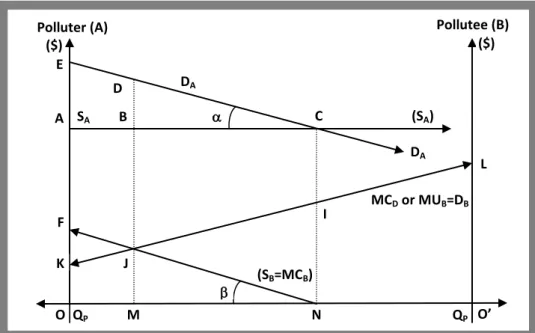
The transaction pertaining to this case may be defined and solved graphi-cally as follows (Fig. 1): We have two superposed axes systems: the one from O rightward to O’ (pertaining to the polluter A) the other from O’ leftward to O (pertaining to the pollutee B.) On each “Y” axes (one pertaining to the polluter A and the other to the polluter B) we have monetary units to measure price, marginal pollution damage cost and marginal utility of pollution decrease. For convenience the upward (increasing) or downward (decreasing) sloping of the curves are indicated by arrows. For example, the demand of A for PP (DA) is a
Figure 1: The Case 1. The Polluter has the Property Right; The Polluter is a Consumer; The
Technology is Invariable.
The arrow of the marginal damage cost MCD (KL) is bidirectional. From
O to O’ the function MCD is upward and rightward sloping indicating the
in-creasing marginal pollution damage cost. But from O’ to O the same function is downward and leftward sloping indicating the decrease of pollution damage cost. As mentioned above the decrease of pollution is utility for B. Therefore this function is leftward and downward sloping indicating the marginal utility or the demand of the pollutee B (MUB=DB) for less pollution damage cost as it
were. On the bidirectional “x” axis, we have the quantity of the pollutant PP
consumed. On the first axis system (from O to O’) we have the downward slop-ing demand DA of the person A for the pollutant PP and the supply curve of the
pollutant PP. The latter one is a horizontal function depending on the assumption
that A is a small competitive buyer who cannot change market price by buying more or less. The supply curve is also the marginal cost of consumption of PP to
the person A.
Having the demand curve (DA) and the supply curve (SA) we can now
de-termine the equilibrium amount of consumption of the person A of the product
(SA)
Polluter (A) Pollutee (B)
($) ($) E A F K O QP D SA B DA J M N QP O’ L C I MCD or MUB=DB DA (SB=MCB)
PP: At the point C the amount bought and consumed equals to ON. We know
that the decrease of consumption of the person A of the product PP decreases the
pollution damage cost inflicted on the pollutee B and thereby increases his/her utility. For example, when consumption is decreased from N to M, the total utility gained by B is MNIJ. Because this is the area under the marginal pollu-tion damage cost curve MCD (integral of the function MCD). By the same token
when A ceases all consumption, the total utility gained by B becomes ONIK. In this first case we assumed that the polluter has the property right. Ac-cordingly, he/she is candidate to receive an amount of compensation from the pollutee to be convinced to decrease or cease the consumption engendering pollution. We also assumed that when a part or the whole of the consumer sur-plus is paid to the polluter A, he/she will unquestionably agree to cease or de-crease his/her consumption. Now it’s time to determine the amount of indemni-ty that the pollutee B should pay to the polluter A. The point where the con-sumption decrease should start is the point N, because this is the maximum amount of consumption A makes when he/she is at equilibrium at the point C.
Now let’s draw from N leftward and upward a line parallel to DA, the
per-son A’s demand curve for PP (this line is drawn by having α = β, fig. 1). By
doing this we get the line NF and a triangle ONF equal to the consumer surplus ACE of the person A. This NF becomes the curve showing the marginal indem-nity cost the person B should pay to the person A. In other words this is the “indemnity supply curve” (SB) or the function showing the amount of indemnity
the person B should pay. By definition, the marginal indemnity cost increases when B pays to A ever growing parts of consumer surplus when consumption and consumer surplus decrease (marginal consumer surpluses.)
As an extreme case, the pollutee B may pay as indemnity the whole of the consumer surplus of A which is the area ACE (by definition equal to ONF) where A will presumably forgo all of consumption of PP. But B will not go so
far because there he/she will incur a total cost greater than the total utility he obtains: when the consumption is reduced to a level beyond the point M where MUB=MCB, the marginal cost of indemnity MCB will become greater than the
marginal utility of B (MUB). The best point that the consumption should be
reduced to is the point M. Because, the point J is the point where the demand of the person B (DB) equals to his/her supply (SB). Therefore, J is the equilibrium
pollution (MUB) becomes equal to the marginal cost of indemnity MCB he/she
should pay.
Now that we have precisely determined the equilibrium of the person A and of the person B, we may also (graphically) measure the exact welfare effect of the transaction between the two transacting parties. The polluter A’s welfare remains exactly the same: his welfare decreases by the amount of decreased consumer surplus (BCD), but he is fully indemnified by the amount of his/her loss (MNJ). Therefore, he/she is indifferent (he/she may also cash a small bonus for an absolute conviction.) As to the pollutee B: when the consumption is de-creased to the point M the total utility he gets from the reduction of the damage is MNIJ. But he only pays the amount MNJ (=BCD). So, even after paying an indemnity he/she still enjoys a net increase in his/her welfare which is NIJ. Let’s note that this conclusion will hold as long as the marginal pollution dam-age cost function MCD) is under (less than) the demand (DA) and supply
func-tions (SA) for the pollutant, as is presumed in figure 1. Like argued above the
person A may also require an amount of bonus in excess of the indemnity paid exactly equal to the consumer surplus lost. The exact determination of the amount of this bonus is outside the framework of this article.
2.1.1.2. Case Two: The Polluter has the Property Right; The Polluter is a Consumer; The Technology is Variable.
When the technology is variable, instead of the marginal indemnity cost curve (SB=MCB) for the pollutee B, we have the marginal cleaning cost curve
MCCL. Therefore the graphical analysis we use in this case has a modification:
here instead of having the B’s supply function SB showing the marginal amount
of indemnity MCB he/she should pay, we have another supply curve RF
representing the cleaning supply function SCL or the marginal cost of cleaning
MCCL to be financed by B (Fig. 2 below).
The supply curve of the person B in relation to the indemnity payment he/she should make to A (as in the case 1) and the supply curve in relation to the cleaning cost (SCL=MCCL) should not be confused. Even though they may
look alike they are completely different. From N leftward to O the pollution damage is decreased by paying a cleaning cost represented by the supply curve RF which is the marginal cleaning cost MCCL. RF is to the origin O’ an upward
maximum) leftward more and more cleaning is made, the marginal cost increas-es. The reason is that the cleaning presumably applies to an already existing pollution with a view to decrease it. In other words the cleaning starts from the point N and proceeds leftward with respect to O’. And again presumably more and more cleansing and purification will require ever increasing cleaning out-lays indicating increasing marginal cleaning cost MC.
Figure 2: The Case 2. The Polluter has the Property Right; The Polluter is a Consumer; the
Technology is Variable.
In this case 2 above, the polluter (A) consumes the amount ON as deter-mined by his/her demand for the good DA and the supply of the good SA. The
pollution damage is represented by the same function KL (MCD). The reverse of
this function (leftward LK) which represents reduction of pollution is the mar-ginal utility and the demand function (MUB=DB) for the person B as explained
before. When the pollutee agrees to pay the marginal cleaning cost starting from N leftward he/she will pay increasingly according to marginal terms. In other words, for every consecutive unit he pays an increasing amount equal to the marginal cleaning cost (e.g. the first marginal payment is NR). Now the equili-brium of the pollutee B becomes established at J where his/her marginal utility
Polluter (A) Pollutee (B)
($) ($) E A F K O QP SA DA R J P N QP O’ L C I MCD or MUB=DB DA (SCL=MCCL) (SA) (SCL=MCCL)
of pollution reduction MUB is equal to the marginal cost of cleaning MCCL. J is
actually the optimum point, because past J the marginal cost of cleaning MCCL
becomes greater than the marginal utility of pollution reduction MUB so that
person B incurs a loss.
What happens at N? The polluter continues to consume the same amount of the product which is ON; the amount of damage prevented is PNIJ; the total cost incurred is PNRJ. Therefore, the pollutee has a utility surplus of RIJ (=PNIJ-PNRJ). Here, only when the marginal cleaning cost is low enough the pollutee will enjoy the total amount of utility (RIJ). But if ever the marginal cleaning cost is higher, the area RIJ will shrink and the net utility will become smaller.
In this case 2 there also remains a residual pollution damage cost which is OPJK. Is it possible to provide some remedy for this residual pollution? Past the point P, more cleaning burdens a loss on the pollutee. So, it is not possible to proceed with more cleaning. The pollutee cannot either offer an indemnity to the polluter to make him/her decrease consumption, because consumption is full and already at N. Therefore here the residual pollution is unavoidable unless the marginal cleaning cost is low enough to let the pollutee proceed with thorough cleansing.
2.1.2. Cases where the Polluter has the Property Right and is a Producer
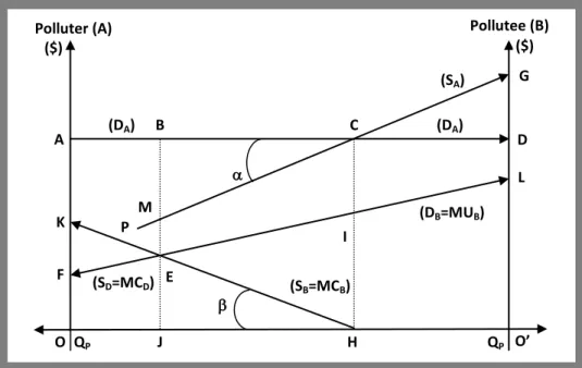
For the polluter who is a producer we may take the example of a cement factory inflicting harm on a touristic hotel in the neighborhood. When the pollu-ter is a producer the graphical analysis and the assumptions change accordingly: The assumptions in relation to this case are the following:
1- The producer’s supply curve is a normal upward sloping curve and it does not include the normal profit (which is the opportunity cost of doing business.) Therefore the producer’s surplus which is the differ-ence (the area) between the demand curve (the marginal revenue curve) and the supply curve (marginal cost curve) reflects the sum of economic profit and normal profit;
2- The market demand curve directed to the producer’s good is flat, meaning that the producer is a perfectly competitive firm which takes the market price,
3- The producer produces for the sole reason of getting an amount of producer’s surplus which is equal to total profit (which is the sum of economic profit and normal profit.)
4- The production inflicts negative externalities as pollution and the mar-ginal pollution damage cost MCD (=SD) is an increasing function.
When the polluter is a producer having the property right again two alter-native cases will be considered:
1- The case where the technology is invariable; 2- The case where the technology is variable.
In the first case, the damage cost can be reduced only when the produc-tion is cut back. Presumably, the producproduc-tion will be cut back provided that the producer is compensated for the producer’s surplus (economic + normal profit) he/she looses. Here like the cases above one may argue that the producer who has the property right may require, apart from the indemnity equal to the pro-ducer’s surplus foregone, an amount of extra in order to be convinced to cut back production. In the second case, the damage cost can be reduced by using a cleaning technology and financing its cost.
2.1.2.1. Case 3: The Polluter has the Property Right; the Polluter is a Producer; the Technology is Invariable
In this case graphically described below (Fig. 3), the production of a good causes a negative externality generating a damage cost which is shown by the marginal damage cost curve MCD (FL in Fig 3.) In the opposite direction (LF)
the same damage cost function is for the pollutee (the person B) a marginal utility function (MUB) for the reasons explained above.
This graphical analysis may be carried out similarly to the case 1. The demand curve directed to the producer’s product is AD (or DA) and his/her
supply curve is PG (SA). The equilibrium of the producer is at C where the
de-mand for his/her product (AD) and his/her supply of product (PG) cross each other. At the equilibrium point C the amount OH is produced. The pollution
damage cost inflicted by the production is represented by FL which is the mar-ginal pollution damage cost (MCD). This is (in regard to the origin O) a
normal-ly rightward and upward sloping suppnormal-ly curve meaning that marginal pollution damage cost is increasing. Leftward with regard to the origin O’ this same curve LF is also the marginal utility or the demand curve (MUB=DB) of the person B
for less pollution as it were.
Figure 3: Case 3. The Polluter has the Property Right; The Polluter is a Producer; The
Technolo-gy is Invariable.
According to our assumption the polluter should accept the indemnity (plus a small amount of bonus) offered to him/her in exchange for his/her reduc-ing or ceasreduc-ing the production. So startreduc-ing from the point H leftward we draw an indemnity supply curve (HK: SB=MCB) designed to determine the amount of
indemnity that the pollutee B should pay to the polluter A. The line is drawn at the slope tg β exactly equal to the slope of producer’s supply curve which is tg α.
The pollutee B reaches his/her equilibrium at E where his/her demand DB
equals the supply or the function indicating the amount of indemnity he/she
Polluter (A) Pollutee (B)
($) ($) B A K F O QP (DA) E J H QP O’ L C I (DB=MUB) (SB=MCB) (DA) (SD=MCD) P (SA) G D M
should pay to the polluter (SB), or MCB=MUB. He/she actually pays the amount
JHE which is exactly equal to MCB, the amount of producer’s surplus foregone by the polluter in exchange for an indemnity of the same amount. After paying the indemnity the total utility obtained by the person B is JHIE which is the amount of pollution damage cost avoided. The cost incurred to him/her by pay-ing the indemnity is JHE. So the welfare of the polluter does not change, be-cause he/she is fully indemnified for the producer’s surplus (economic plus normal profit) he/she looses; but the pollutee has the surplus of HIE (=JHIE-JHE) even after paying the indemnity (Fig 3.)
2.1.2.2. Case 4: The Polluter has the Property Right; The Polluter is a Producer; The Technology is Variable
Here, most of the elements of the graphics are like those of the previous case, except that in the figure 4 below instead of marginal indemnity cost curve MCB we have the marginal cleaning cost MCCL. This curve FG starts at the
pro-duction level H. The marginal cost of cleaning at H is HF. To the origin O’ this curve is leftward and upward sloping meaning that starting from production point H leftwards we have an increasing marginal cleaning cost MCCL which is
also the cleaning supply curve for the person B (SB). In this case we need some
additional assumptions: as compared to the producer’s surplus the cleaning cost should be low enough; otherwise the pollutee instead of financing the cleaning will prefer to indemnify the producer’s surplus (or the economic and normal profit foregone) of the polluter.
According to the assumptions set forth above starting from the point H until J the marginal cleaning cost (MCCL) is smaller than the marginal damage
cost MCD (at the outset; HF <HB.). Therefore, up until J it is worthwhile for the
pollutee to finance cleaning. When we reach the equilibrium at E (DB=SB) the
welfare situation becomes as follows: The pollution damage represented by the area JHBE is fully avoided by cleaning. The cost of the cleaning is the area JHFE which is smaller than JHBE. Therefore, the net welfare increase for the pollutee who finances the cleaning is FBE (JHBE- JHFE).
Figure 4: Case 4. The Polluter has the Property Right; The Polluter is a Producer; The
Technol-ogy is Variable.
So here, under the assumption that up until the equilibrium point E the marginal cleaning cost (FE) is less than (under) the marginal damage cost (EB), the pollutee will be better off by financing the cleaning. Otherwise instead of financing the cleaning he/she, like in the case 3, will prefer to pay the produc-er’s surplus up until J (which is MCI.) In view of the equilibrium of the person B, the cleaning is possible up until the point J. Once that the cleaning alternative is chosen, past the point J the pollutee cannot choose to pay the remaining pro-ducer’s surplus in order to reduce more pollution and damage because in the cleaning case the production level remains at the starting point H.
2.2. Cases where the Pollutee has the Property Right
Now we consider the cases where it is not legally or anyhow warranted to carry out an activity causing pollution. For the polluter who is a consumer the example given above (the consumer burns a pollutant such as wood) also holds here. For the polluter who is a producer we may take again the example of a cement factory inflicting harm on a touristic hotel in the neighborhood. Here the
Polluter (A) Pollutee (B)
($) ($) I A G P O QP (DA) E J H QP O’ L C B (DB=MUB) SB=MCCL (DA) (SB=MCCL) (SA) N D F M (SD=MCD) (SA)
cement factory which does not have the property right has an alternative: it can either indemnify the hotel for the profit reduced due to pollution or construct chimney filters in order to prevent pollution. It goes without saying that the pollutee will agree not to file a complaint when he/she is duly indemnified by the polluter.
2.2.1. Cases where the Pollutee has the Property Right and the Pollu-ter is a Consumer
The first case under this heading is the situation where we have an invari-able technology in which we don’t have any cleaning possibility.
Figure 5: The Case 5. The Pollutee has the Property Right; The Polluter is a Consumer; The
Technology is Invariable.
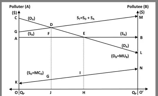
2.2.1.1. Case 5. The Pollutee has the Property Right; The Polluter is a Consumer; The Technology is Invariable
This case is graphically described in figure 5 above. There, CL is the de-mand of the consumer for the good which is a pollutant. The curve AB is the
Polluter (A) Pollutee (B)
($) ($) F A K O QP (SA) G J H QP O’ L E I (DB=MUB) ST=SD + SA (DA) (SD=MCD) (SA) M B D C G N (DA)
supply curve of the consumer, indicating the amount of money he/she should pay to consume the good. The consumer is fully competitive he/she cannot change the market price so the supply curve is fully flat. On the other hand, the curve KN is the marginal pollution damage cost which is an increasing function which means that when the consumption increases the marginal pollution dam-age cost of each additional consumption unit also increases. In the reverse direc-tion from N to K, the same curve is actually a marginal utility and a demand curve (MUB=DB) for the pollutee B, because any reduction of pollution damage
cost is indeed an amount of utility for the pollutee.
When we disregard the externality KN, the consumer is at equilibrium at E and consumes the amount OH. But given that the pollutee B has the property right the pollution damage inflicted on him/her should be paid by the polluter who in this case is a consumer. Therefore in order to internalize the external cost we vertically add the marginal pollution damage cost curve KN (SD) curve
onto the normal supply curve AB (SA which is the internal marginal cost of the
consumer) and we get the total supply curve ST (GM) which faces the polluter
A.
With the new total supply curve (ST=SD+SA), the new equilibrium for the
polluter becomes established at D. There, due to the increase of the marginal cost the consumer decreases his/her consumption to OJ. At the consumption level OJ the polluter also pays as indemnity the full amount of pollution damage cost OJGK equal to AFDG. Due to the decrease of consumption from the point H to the point J the person looses the amount of consumer surplus FED. What becomes to the welfare of each party after the settlement? The pollutee’s dam-age cost OJGK is covered by the indemnity AFDG (=OJGK) he gets from the person A, so he/she is indifferent. The polluter who consumes the pollutant by the amount OJ gets a consumer surplus by the amount AFDC. The part AFDG of AFDC is paid to the pollutee as indemnity. Despite this, the polluter still enjoys an amount of consumer surplus which is GDC. Here again the transac-tion depends upon the height of the pollutransac-tion damage. When the pollutransac-tion dam-age and the indemnity to pay are high, the polluter who is a consumer may pre-fer not to consume the pollutant at all.
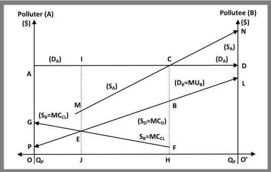
2.2.1.2. Case 6. The Pollutee has the Property Right; The Polluter is a Consumer; The Technology is Variable
Here again instead of having a marginal pollution damage cost curve we have a marginal cleaning cost curve which reflects the cleaning supply SCL (KI
in Fig 6 below). The marginal cleaning cost function or the cleaning supply curve is different from the marginal damage cost curve. Therefore the welfare effects in this case are also different from those of the previous case. The pollu-ter who does not have the property right is obliged to clean the pollution. There-fore differently from case 4, here the cleaning starts at the outset of the con-sumption beginning at the point O. The cleaning supply curve SCL reflects the
amount of marginal cleaning cost faced by the consumer/polluter. That is why the cleaning supply is to the origin O upward and leftward sloping.
Figure 6. The Case 6. The Pollutee has the Property Right; The Polluter is a Consumer; The Technology is Variable.
Here the polluter consumes a pollutant for which his/her demand is ML. His/her supply curve for the polluter is AB. So, his/her equilibrium is at G. There he/she consumes the amount OH. But this consumption causes an
exter-Polluter (A) Pollutee (B)
($) ($) F A K O QP (SA) L J H QP O’ L G I (ST=SA + SCL) (DA) (SCL=MCCL) (SA) M B E M C (DA) D
nality which we do not have to show here. Because once the cleaning is fi-nanced the whole pollution damage becomes avoided. Given that the technology is variable, the polluter who does not have the property right should finance the cleaning costs.
The supply curve in relation to the cleaning is KI. It is an increasing mar-ginal cost to the origin O. In order to establish the new equilibrium we vertically add the cleaning supply curve or the marginal cleaning cost curve KI (SCL) to
the consumer’s supply curve AB (SA) and we get the total supply curve CD
(ST=SA+SCL) which faces the consumer/polluter. When we get together the total
supply curve ST and the demand curve DA we reach a new equilibrium point E.
At E, the consumer’s consumption recedes from OH to OJ. And due to in-creased cost, he/she foregoes the amount JH and his consumer’s surplus de-creases from AGM to AFEM. In order to be able to consume the amount OJ, he/she covers the total cost of cleaning OJLK which is equal to AFEC.
Now, what is the welfare outcome of this arrangement? The polluter con-suming the amount OJ instead of OH looses the amount of FGE (and AFEC) of the consumer surplus. But, he/she continues to enjoy the amount of consumer surplus CEM. Because from the remaining consumer surplus AFEM, we deduct the amount of cleaning cost which is AFEC equal to OJLK. Here we clearly see that the amount of remaining consumer surplus depends on the amount of the cleaning cost. When the cleaning cost is low enough the consumer may enjoy a larger amount of consumer surplus. Here the amount of the damage cost is not relevant. It may be lower or higher than the cleaning cost. What matters is the cleaning which avoids the whole damage cost. When the cleaning cost is too high the consumer/polluter instead of financing the cleaning cost may prefer to indemnify the pollutee for the pollution damage like in case 5.
2.2.2. Cases where the Pollutee has the Property Right and the Pol-luter is a Producer
The example for the case where the polluter is a producer is the cement factory inflicting harm to a touristic hotel (already given above.) In this situation we again have two alternative cases where the technology is invariable or varia-ble.
Figure 7. Case 7. The Pollutee has the Property Right; The Polluter is a Producer; The
Technol-ogy is Invariable.
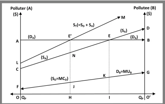
2.2.2.1. Case 7. The Pollutee has the Property Right; The Polluter is a Producer; The Technology is Invariable
When the technology is invariable the polluter may either give up produc-tion or may offer an indemnity to the pollutee holding the property right. In the figure 7 above we see the graphical solution to the case where the technology is invariable. Here again, the producer produces a good (such as cement) which causes pollution in the production process. Presumably there is a horizontal market demand AB for the good reflecting the fact that the producer is a per-fectly competitive firm which cannot change the market price. This producer has also a supply curve CD which (to the origin O) is a normal rightward and upward sloping supply curve reflecting increasing marginal production costs. Disregarding the externality, the producer is at equilibrium at E where he/she produces and sells the amount OI. He/she also earns a producer’s surplus CEA which is equal to total profit (economic profit + normal profit) as explained before.
Polluter (A) Pollutee (B)
($) ($) E’ A F O QP (SA) J I H QP O’ E K DB=MUB ST(=SD + SA) (DA) (SD=MCD) (SA) D B C L G (DA) M N
The pollution the producer causes has a marginal damage cost MCD (FG).
So the total amount of damage cost inflicted by the production is OIKF. Given that the producer (the person A) does not have property right, he/she is not al-lowed to inflict this damage. Therefore he/she has to indemnify the pollutee B for the damage he/she causes. For example when the amount OI is produced the amount of indemnity that he/she should pay becomes equal to the total amount of the damage cost which is OIKF, but he/she cannot afford it. When the pollu-ter decides to indemnify the pollutee B, equilibrium conditions change. The marginal damage cost is internalized by vertically adding the marginal damage cost MCD (FG) onto the normal supply curve SA (CD) of the producer A. Then
the supply curve SA (CD) shifts and becomes the total supply curve ST (=SA+SD)
which is LM. Due to the upward shift of the supply curve the equilibrium of the producer recedes to E’ and due to higher marginal costs the production decreas-es from I to H. At H the remaining pollution damage cost is OHJF.
As to the welfare change: the amount of CNE’L (=OHJF) is paid to the pollutee B as damage indemnity. So, B becomes indifferent. The producer loos-es the portion of CEE’L (=CEA-LE’A) of the producer’s surplus. But he/she still enjoys the amount of producer’s surplus LE’A. Of course this outcome depends upon the amount of the pollution damage cost or the amount of indem-nity. When this amount increases the producer’s surplus shrinks. Presumably, it is the component of economic profit of the producer’s surplus which first de-creases (remember that we excluded the normal profit from the supply curve and included into the producer’s surplus). Therefore the polluter, who here is the producer, may continue to produce until the producer’s surplus becomes equal not to zero but solely to the normal profit or the opportunity cost of this business; and there the producer gets the long run equilibrium. Given that it is not possible to show the amount of normal profit, here we cannot graphically show until where the production recedes.
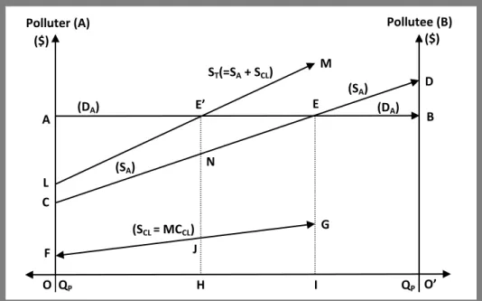
2.2.2.2. Case 8. The Pollutee has the Property Right; The Polluter is a Producer; The Technology is Variable
In this last case where the technology is variable, instead of the marginal pollution damage cost function we again have the marginal cleaning cost func-tion (the cleaning supply funcfunc-tion). Because when the cleaning is done all pollu-tion becomes avoided, therefore there is no need to show the pollupollu-tion damage
function. In the figure 8 below we have all the elements of the case 7 except that instead of the marginal pollution damage function (MCD) we have the marginal
cleaning cost function (MCCL) because the polluter is obliged to clean up. So the
total supply is formed by the vertical addition of the usual supply function SA
(CD) and the cleaning supply function SCL (FG) which is the marginal cleaning
cost function (MCCL). Therefore, by adding the two we internalize the cleaning
cost.
The total supply function ST (=SA+SCL) is LM and the new equilibrium is
at E’. The production is reduced from I to H. The damage is fully eliminated by cleaning and the cost of cleaning is OHJF. The cleaning cost is internalized as CNE’L which is financed by the polluter who does not have the property right. As to the welfare effect: the producer’s surplus recedes from CEA to CNE’A. The portion CNE’L of CNE’A is paid off as the cleaning cost and the net re-maining producer’s surplus becomes LE’A. Of course, this effect depends upon the amount of the cleaning cost. When the cleaning cost is too high, the produc-er’s surplus will shrink.
Figure 8: Case 8. The Pollutee has the Property Right; The Polluter is a Producer; The
Technol-ogy is Variable.
Polluter (A) Pollutee (B)
($) ($) E’ A F O QP (SA) J I H QP O’ E ST(=SA + SCL) (DA) (SCL = MCCL) (SA) D B C L G (DA) M N
Here like in the case 7 the producer may go as far as the remaining pro-ducer’s surplus becomes equal to the normal profit where the economic profit is zero. Past this point the producer is expected to give up business. Again like in the other cases where the cleaning cost is relatively high and the pollution dam-age cost is low the polluter may try to bribe the pollutee by paying an indemnity equal to the amount of damage which he/she inflicts on him/her.
Discussion on the Validity of the Assumptions and on the Limitations In this article, transaction costs are assumed as zero, like Coase did. Here I have nothing to add on the debates about the validity of zero transaction costs. On the other hand, the relevant assumptions are specified in each specific case. As to the validity of the assumptions: the assumption that a consumer consumes anything in order to get a consumer surplus and that a producer produces in order to get a producer’s surplus are reasonable and holds in economics. Actual-ly, in the theory and practice of cost-benefit analysis, consumer and producer surpluses are taken as the sole measures of welfare. Our proposition to deduct the normal (marginal) profit from the supply curve is also reasonable. I don’t think this will distort the marginal cost curves.
Here like in any topic of microeconomics and public sector economics measurement difficulties may be relevant. In other words the cases or models described in this article may be criticized for not having the ability to be meas-ured. For example, how can we measure consumer and producer surpluses in order to determine the amount of indemnity? There are also measurement diffi-culties as far as the pollution damage cost is concerned. When the pollutee has the property right and should be indemnified we should be able to measure the marginal pollution damage cost. Actually measurement difficulties always exist in microeconomics and in cost-benefit analysis. When we insistently require the ability of being measured there will remain very few topics in microeconomics, public economics and specifically cost-benefit analysis that can studied. There-fore I have nothing to propose on the measurement problems.
In this article I only took the cases where the polluters alternatively were consumers and producers. There was no specification about the status of the pollutees. Actually even the pollutees may alternatively be consumer or produc-ers. Then the marginal pollution damage cost inflicted on them may be
materia-lized as reduction in their consumer’s surplus or producer’s surplus. So, proba-bly this article may need to be completed by defining the status of the pollutees.
Summary
In this article originally developed upon the old idea of Professor Ronald Coase, I generalized all the possible cases of Coasean transactions and analyzed the welfare effects of each. In order to determine all the possible cases I took three dichotomies into account: the identity of the polluter as being consumer or producer; the legal status of the polluter or the pollutee as having the property right or not having the property right; the technology of consumption or produc-tion as being invariable (meaning that there is no possibility of cleaning) or variable (meaning that there is a possibility of cleaning.) Taking the combina-tion of all those dichotomies I determined eight different cases like as follows: case 1: the polluter has the property right; the polluter is a consumer; the tech-nology is invariable; case 2: the polluter has the property right; the polluter is a consumer; the technology is variable; case 3: the polluter has the property right; the polluter is a producer; the technology is invariable and the following…
Each and every one of the cases was graphically analyzed, its equilibrium and welfare effects was graphically determined. This graphical approach made possible to determine the exact amount of indemnity (in graphics) that persons who do not have property right should pay to their transacting counterparts. In this article it was seen that the polluters or the pollutees who did not have the property right may also take advantage (as welfare increase) of the transactions even in the case of paying the indemnity.
The choice of the payers either on financing the indemnity or alternative-ly the cleaning cost depends upon the relative amounts of the marginal pollution damage costs and the marginal cleaning costs. When the cleaning costs are higher the polluters who don’t have the property right may prefer to pay the pollution damage cost. In each case, it was also proved that there was usually a possibility of agreement profitable to both sides. This article also provided pre-cise graphical equilibrium solutions for both the polluters and the pollutees in Coasean transactions.
FOOTNOTES and REFERENCES 1
Coined word meaning put forth by Professor R.H. Coase
2
Coined word meaning harmed by pollution
3
Coase, R.H., The Problem of Social Cost, Journal of Law and Economics, 1960
4
A.C. Pigou, The Economics of Welfare, 1920
5
Coined word meaning put forth by Professor A.C. Pigou
6Stigler, G. The Theory of Price, 1966 7