Angular analysis of Bd0 → K ∗ μ + μ − decays in pp collisions at √s=8 TeV with the ATLAS detector

JHEP10(2018)047

Published for SISSA by Springer

Received: May 11, 2018 Revised: September 5, 2018 Accepted: September 27, 2018 Published: October 8, 2018

Angular analysis of B

_d

0

→ K

∗

µ

+

µ

−

decays in pp

collisions at

√

s = 8 TeV with the ATLAS detector

The ATLAS collaboration

E-mail:

atlas.publications@cern.ch

Abstract: An angular analysis of the decay B

d0

→ K

∗

µ

+

µ

−

is presented, based on

proton-proton collision data recorded by the ATLAS experiment at the LHC. The study is

us-ing 20.3 fb

−1

of integrated luminosity collected during 2012 at centre-of-mass energy of

√

s = 8 TeV. Measurements of the K

∗

_{longitudinal polarisation fraction and a set of}

angu-lar parameters obtained for this decay are presented. The results are compatible with the

Standard Model predictions.

Keywords: Hadron-Hadron scattering (experiments)

JHEP10(2018)047

Contents

1

Introduction

1

2

Analysis method

2

3

The ATLAS detector, data, and Monte Carlo samples

4

4

Event selection

4

5

Maximum-likelihood fit

6

5.1

Signal model

7

5.2

Background modes

8

5.3

K

∗

cc control sample fits

10

5.4

Fitting procedure and validation

11

6

Results

11

7

Systematic uncertainties

18

8

Comparison with theoretical computations

21

9

Conclusion

23

A Correlation matrices

24

The ATLAS collaboration

30

1

Introduction

Flavour-changing neutral currents (FCNC) have played a significant role in the construction

of the Standard Model of particle physics (SM). These processes are forbidden at tree level

and can proceed only via loops, hence are rare. An important set of FCNC processes involve

the transition of a

b-quark to an sµ

+

_µ

−

_{final state mediated by electroweak box and penguin}

diagrams. If heavy new particles exist, they may contribute to FCNC decay amplitudes,

affecting the measurement of observables related to the decay under study. Hence FCNC

processes allow searches for contributions from sources of physics beyond the SM (hereafter

referred to as new physics). This analysis focuses on the decay

B

0

d

→ K

∗0

_(892)µ

+

_µ

−

_{, where}

K

∗0

(892) →

K

+

_π

−

_{. Hereafter, the}

_K

∗0

_{(892) is referred to as}

_K

∗

_{and charge conjugation}

is implied throughout, unless stated otherwise. In addition to angular observables such

JHEP10(2018)047

as the forward-backward asymmetry

A

FB

,

1

there is considerable interest in measurements

of the charge asymmetry, differential branching fraction, isospin asymmetry, and ratio of

rates of decay into dimuon and dielectron final states, all as a function of the invariant

mass squared of the dilepton system

q

2

_{. All of these observable sets can be sensitive to}

different types of new physics that allow for FCNCs at tree or loop level. The BaBar, Belle,

CDF, CMS, and LHCb collaborations have published the results of studies of the angular

distributions for

B

0

d

→ K

∗

_µ

+

_µ

−

_[

₁

_–

₈

_{]. The LHCb Collaboration has reported a potential}

hint, at the level of 3.4 standard deviations, of a deviation from SM calculations [

3

,

4

]

in this decay mode when using a parameterization of the angular distribution designed

to minimise uncertainties from hadronic form factors. Measurements using this approach

were also reported by the Belle and CMS Collaborations [

6

,

8

] and they are consistent

with the LHCb experiment’s results and with the SM calculations. This paper presents

results following the methodology outlined in ref. [

3

] and the convention adopted by the

LHCb Collaboration for the definition of angular observables described in ref. [

9

]. The

results obtained here are compared with theoretical predictions that use the form factors

computed in ref. [

10

].

This article presents the results of an angular analysis of the decay

B

0

d

→ K

∗

_µ

+

_µ

−

with the ATLAS detector, using 20.3 fb

−1

of

pp collision data at a centre-of-mass energy

√

s = 8 TeV delivered by the Large Hadron Collider (LHC) [

11

] during 2012. Results are

presented in six different bins of

q

2

_{in the range 0.04 to 6.0 GeV}

2

_{, where three of these bins}

overlap. Backgrounds, including a radiative tail from

B

0

d

→ K

∗

J/ψ events, increase for q

2

above 6.0 GeV

2

, and for this reason, data above this value are not studied.

The operator product expansion used to describe the decay

B

0

d

→ K

∗

µ

+

µ

−

encodes

short-distance contributions in terms of Wilson coefficients and long-distance contributions

in terms of operators [

12

]. Global fits for Wilson coefficients have been performed using

measurements of

B

0

d

→ K

∗

µ

+

µ

−

and other rare processes. Such studies aim to connect

deviations from the SM predictions in several processes to identify a consistent pattern

hinting at the structure of a potential underlying new-physics Lagrangian, see refs. [

13

–

15

].

The parameters presented in this article can be used as inputs to these global fits.

2

Analysis method

Three angular variables describing the decay are defined according to convention described

by the LHCb Collaboration in ref. [

9

]: the angle between the

K

+

_{and the direction opposite}

to the

B

0

d

in the

K

∗

centre-of-mass frame (θ

K

); the angle between the

µ

+

and the direction

opposite to the

B

0

d

in the dimuon centre-of-mass frame (θ

L

); and the angle between the two

decay planes formed by the

Kπ and the dimuon systems in the B

0

d

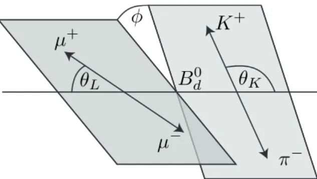
rest frame (φ). For B

0 d

mesons the definitions are given with respect to the negatively charged particles. Figure

1

illustrates the angles used.

1_{The forward-backward asymmetry is given by the normalised difference between the number of positive}

muons going in the forward and backward directions with respect to the direction opposite to B0

dmomentum

JHEP10(2018)047

φ

B

_d0

µ

+

µ

−

K

+

π

−

θL

θ

K

Figure 1. An illustration of theB0

d → K∗µ+µ− decay showing the anglesθK, θL and φ defined

in the text. Angles are computed in the rest frame of the K∗, dimuon system and B0

d meson,

respectively.

The angular differential decay rate for

B

0 d

→ K

∗

_µ

+

_µ

−

_{is a function of}

_q

2

_{, cos}

_θ

K

, cos

θ

L

and

φ, and can be written in several ways [

16

]. The form to express the differential decay

amplitude as a function of the angular parameters uses coefficients that may be represented

by the helicity or transversity amplitudes [

17

] and is written as

2

1

dΓ/dq

2

d

4

Γ

d cos

θ

L

d cosθ

K

dφdq

2

=

9

32π

"

3(1−

F

L

)

4

sin

2

_θ

K

+F

L

cos

2

θ

K

+

1−F

L

4

sin

2

_θ

K

cos 2θ

L

−F

L

cos

2

θ

K

cos 2θ

L

+S

3

sin

2

θ

K

sin

2

θ

L

cos 2φ

+S

4

sin 2θ

K

sin 2θ

L

cosφ+S

5

sin 2θ

K

sinθ

L

cos

φ

+S

6

sin

2

θ

K

cosθ

L

+S

7

sin 2θ

K

sin

θ

L

sin

φ

+S

8

sin 2θ

K

sin 2θ

L

sin

φ+S

9

sin

2

θ

K

sin

2

θ

L

sin 2φ

#

.

(2.1)

Here

F

L

is the fraction of longitudinally polarised

K

∗

mesons and the

S

i

are angular

coefficients. These angular parameters are functions of the real and imaginary parts of the

transversity amplitudes of

B

0

d

decays into

K

∗

_µ

+

_µ

−

_{. The forward-backward asymmetry is}

given by

A

FB

= 3S

6

/4. The predictions for the S parameters depend on hadronic form

factors which have significant uncertainties at leading order. It is possible to reduce the

theoretical uncertainty in these predictions by transforming the

S

i

using ratios constructed

to cancel form factor uncertainties at leading order. These ratios are given by refs. [

17

,

18

] as

P

1

=

2S

3

1 −

F

L

(2.2)

P

2

=

2

3

A

FB

1 −

F

L

(2.3)

P

3

= −

S

9

1 −

F

L

(2.4)

P

_j=4,5,6,80

=

S

i=4,5,7,8

pF

L

(1 −

F

L

)

.

(2.5)

2_{This equation neglects possible Kπ S-wave contributions. The effect of an S-wave contribution is}

JHEP10(2018)047

All of the parameters introduced,

F

L

,

S

i

and

P

j(0)

, may vary with

q

2

and the data are

analysed in

q

2

_{bins to obtain an average value for a given parameter in that bin.}

3

The ATLAS detector, data, and Monte Carlo samples

The ATLAS experiment at the LHC is a general-purpose detector with a cylindrical

ge-ometry and nearly 4π coverage in solid angle [

19

]. It consists of an inner detector (ID)

for tracking, a calorimeter system and a muon spectrometer (MS). The ID consists of

silicon pixel and strip detectors, with a straw-tube transition radiation tracker providing

additional information for tracks passing through the central region of the detector.

3

The

ID has a coverage of |η| < 2.5, and is immersed in a 2T axial magnetic field generated

by a superconducting solenoid. The calorimeter system, consisting of liquid argon and

scintillator-tile sampling calorimeter subsystems, surrounds the ID. The outermost part of

the detector is the MS, which employs several detector technologies in order to provide

muon identification and a muon trigger. A toroidal magnet system is embedded in the MS.

The ID, calorimeter system and MS have full azimuthal coverage.

The data analysed here were recorded in 2012 during Run 1 of the LHC. The

centre-of-mass energy of the

pp system was

√

s = 8 TeV. After applying data-quality criteria, the

data sample analysed corresponds to an integrated luminosity of 20.3 fb

−1

. A number of

Monte Carlo (MC) signal and background event samples were generated, with

b-hadron

production in

pp collisions simulated with Pythia 8.186 [

20

,

21

]. The AU2 set of tuned

parameters [

22

] is used together with the CTEQ6L1 PDF set [

23

]. The EvtGen 1.2.0

program [

24

] is used for the properties of b- and c-hadron decays. The simulation included

modelling of multiple interactions per

pp bunch crossing in the LHC with Pythia soft

QCD processes. The simulated events were then passed through the full ATLAS detector

simulation program based on Geant 4 [

25

,

26

] and reconstructed in the same way as data.

The samples of MC generated events are described further in section

5

.

4

Event selection

Several trigger signatures constructed from the MS and ID inputs are selected based on

availability during the data-taking period, prescale factor and efficiency for signal

iden-tification. Data are combined from 19 trigger chains where 21%, 89% or 5% of selected

events pass one or more triggers with one, two, or at least three muons identified online

in the MS, respectively. Of the events passing the requirement of at least two muons, the

largest contribution comes from the chain requiring one muon with a transverse momentum

p

T

> 4 GeV and the other muon with p

T

> 6 GeV. This combination of triggers ensures

that the analysis remains sensitive to events down to the kinematic threshold of

q

2

_{= 4m}

2

µ

,

3

ATLAS uses a right-handed coordinate system with its origin at the nominal interaction point (IP) in the centre of the detector and the z-axis along the beam pipe. The x-axis points from the IP to the centre of the LHC ring, and the y-axis points upward. Cylindrical coordinates (r, Φ) are used in the transverse plane, Φ being the azimuthal angle around the z-axis. The pseudorapidity is defined in terms of the polar angle θ as η = − ln tan(θ/2).

JHEP10(2018)047

where

m

µ

is the muon mass. The effective average trigger efficiency for selected signal

events is about 29%, determined from signal MC simulation.

Muon track candidates are formed offline by combining information from both the ID

and MS [

27

]. Tracks are required to satisfy |η| < 2.5. Candidate muon (kaon and pion)

tracks in the ID are required to satisfy

p

T

> 3.5 (0.5) GeV. Pairs of oppositely charged

muons are required to originate from a common vertex with a fit quality

χ

2

_{/NDF < 10.}

Candidate

K

∗

mesons are formed using pairs of oppositely charged kaon and

pion candidates reconstructed from hits in the ID. Candidates are required to satisfy

p

T

(K

∗

)

> 3.0 GeV. As the ATLAS detector does not have a dedicated charged-particle

identification system, candidates are reconstructed with both possible

Kπ mass

hypothe-ses. The selection implicitly relies on the kinematics of the reconstructed

K

∗

meson to

determine which of the two tracks corresponds to the kaon. If both candidates in an

event satisfy selection criteria, they are retained and one of them is selected in the next

step following a procedure described below. The

Kπ invariant mass is required to lie in

a window of twice the natural width around the nominal mass of 896 MeV, i.e. in the

range [846, 946] MeV. The charge of the kaon candidate is used to assign the flavour of the

reconstructed

B

0

d

candidate.

The

B

0

d

candidates are reconstructed from a

K

∗

candidate and a pair of oppositely

charged muons. The four-track vertex is fitted and required to satisfy

χ

2

_{/NDF < 2 to}

suppress background. A significant amount of combinatorial,

B

0

d

,

B

+

,

B

s0

and Λ

b

back-ground contamination remains at this stage. Combinatorial backback-ground is suppressed by

requiring a

B

0

d

candidate lifetime significance

τ /σ

τ

> 12.5, where the decay time

uncer-tainty

σ

τ

is calculated from the covariance matrices associated with the four-track vertex

fit and with the primary vertex fit. Background from final states partially reconstructed

as

B → µ

+

_µ

−

_{X accumulates at invariant mass below the B}

0

d

mass and contributes to the

signal region. It is suppressed by imposing an asymmetric mass cut around the nominal

B

0

d

mass, 5150 MeV

< m

Kπµµ

< 5700 MeV. The high-mass sideband is retained, as the

parameter values for the combinatorial background shapes are extracted from the fit to

data described in section

5

. To further suppress background, it is required that the angle

Θ, defined between the vector from the primary vertex to the

B

0

d

candidate decay vertex

and the

B

0

d

candidate momentum, satisfies cos Θ

> 0.999. Resolution effects on cos θ

K

,

cos

θ

L

and

φ were found to have a negligible effect on the ATLAS B

0s

→ J/ψφ analysis [

28

].

It is assumed to also be the case for

B

0

d

→ K

∗

_µ

+

_µ

−

_.

On average 12% of selected events in the data have more than one reconstructed

B

0 d

candidate. The fraction is 17% for signal MC samples and 2–10% for exclusive background

MC samples. A two-step selection process is used for such events. For 4% of these events it

is possible to select a candidate with the smallest value of the

B

0

d

vertex

χ

2

/NDF. However,

the majority, about 96%, of multiple candidates arise from four-track combinations where

the kaon and pion assignments are ambiguous. As these candidates have degenerate values

for the

B

0

d

candidate vertex

χ

2

/NDF, a second selection step is required. The B

0d

candidate

reconstructed with the smallest value of |m

Kπ

− m

K∗

|/σ(m

_Kπ

) is retained for analysis,

where

m

Kπ

is the

K

∗

candidate mass,

σ(m

Kπ

) is the per-event uncertainty in this quantity,

and

m

K∗

is the world average value of the

K

∗

mass.

JHEP10(2018)047

The selection procedure results in an incorrect flavour tag (mistag) for some signal

events. The mistag probability of a

B

0

d

(B

0

d

) meson is denoted by

ω (ω) and is determined

from MC simulated events to be 0.1088 ± 0.0005 (0.1086 ± 0.0005). The mistag probability

varies slightly with

q

2

_{such that the difference}

_{ω − ω remains consistent with zero. Hence}

the average mistag rate hωi in a given q

2

_{bin is used to account for this effect. If a candidate}

is mistagged, the values of cos

θ

L

, cos

θ

K

and

φ change sign, while the latter two are also

slightly shaped by the swapped hadron track mass hypothesis. Sign changes in these angles

affect the overall sign of the terms multiplied by the coefficients

S

5

,

S

6

,

S

8

and

S

9

(similarly

for the corresponding

P

(0)

_{parameters) in equation (}

_2.1

_{). The corollary is that mistagged}

events result in a dilution factor of (1 − 2hωi) for the affected coefficients.

The region

q

2

_{∈ [0.98, 1.1] GeV}

2

_{is vetoed to remove any potential contamination from}

the

φ(1020) resonance. The remaining data with q

2

_{∈ [0.04, 6.0] GeV}

2

_{are analysed in}

order to extract the signal parameters of interest. Two

K

∗

_{cc control regions are defined for}

B

0

d

decays into

K

∗

_{J/ψ and K}

∗

_{ψ(2S), respectively as q}

2

_{∈ [8, 11] and [12, 15] GeV}

2

_{. The}

control samples are used to extract values for nuisance parameters describing the signal

probability density function (pdf) from data as discussed in section

5.3

.

For

q

2

_{< 6 GeV}

2

_{the selected data sample consists of 787 events and is composed of}

signal

B

0

d

→ K

∗

_µ

+

_µ

−

_{decay events as well as background that is dominated by a}

combina-torial component that does not peak in

m

Kπµµ

and does not exhibit a resonant structure in

q

2

_{. Other background contributions are considered when estimating systematic}

uncertain-ties. Above 6 GeV

2

the background contribution increases significantly, including events

coming from

B

0

d

→ K

∗

J/ψ with a radiative J/ψ → µ

+

µ

−

γ decay. Scalar Kπ contributions

are neglected in the nominal fit and considered only when addressing systematic

uncertain-ties. The data are analysed in the

q

2

_{bins [0.04, 2.0], [2.0, 4.0] and [4.0, 6.0] GeV}

2

_{, where}

the bin width is chosen to provide a sample of signal events sufficient to perform an angular

analysis. The width is much larger than the

q

2

_{resolution obtained from MC simulated}

signal events and observed in data for

B

0

d

decays into

K

∗

_{J/ψ and K}

∗

_{ψ(2S). Additional}

overlapping bins [0.04, 4.0], [1.1, 6.0] and [0.04, 6.0] GeV

2

_{are analysed in order to facilitate}

comparison with results of other experiments and with theoretical predictions.

5

Maximum-likelihood fit

Extended unbinned maximum-likelihood fits of the angular distributions of the signal decay

are performed on the data for each

q

2

_{bin. The discriminating variables used in the fit are}

m

Kπµµ

, the cosines of the helicity angles (cos

θ

K

and cos

θ

L

), and

φ. The likelihood L for

a given

q

2

_{bin is}

L =

e

−n

N !

N

Y

k=1

X

l

n

l

P

kl

(m

Kπµµ

, cos θ

K

, cos θ

L

, φ;

p, b

b

θ),

(5.1)

where

N is the total number of events, the sum runs over signal and background

compo-nents,

n

l

is the fitted yield for the

l

th

component,

n is the sum over n

l

, and

P

kl

is the pdf

evaluated for event

k and component l. In the nominal fit, l iterates only over one signal

JHEP10(2018)047

and one background component. The

p are parameters of interest (F

_b

L

,

S

i

) and b

θ are

nui-sance parameters. The remainder of this section discusses the signal model (section

5.1

),

treatment of background (section

5.2

), use of

K

∗

_{cc decay control samples (section}

_5.3

_),

fitting procedure and validation (section

5.4

).

5.1

Signal model

The signal mass distribution is modelled by a Gaussian distribution with the width given

by the per-event uncertainty in the

Kπµµ mass, σ(m

Kπµµ

), as estimated from the track

fit, multiplied by a unit-less scale factor

ξ, i.e. the width given by ξ · σ(m

Kπµµ

). The mean

values of the

B

0

d

candidate mass (m

0

) and

ξ of the signal Gaussian pdf are determined from

fits to data in the control regions as described in section

5.3

. The simultaneous extraction

of all coefficients using the full angular distribution of equation (

2.1

) requires a certain

minimum signal yield and signal purity to avoid a pathological fit behaviour. A significant

fraction of fits to ensembles of simulated pseudo-experiments do not converge using the

full distribution. This is mitigated using trigonometric transformations to fold certain

angular distributions and thereby simplify equation (

2.1

) such that only three parameters

are extracted in one fit:

F

L

,

S

3

and one of the other

S parameters. For these folding schemes

the angular parameters of interest, denoted by

p in equation (

_b

5.1

), are (F

L

, S

3

, S

i

) where

i = 4, 5, 7, 8. These translate into (F

L

, P

1

, P

j0

), where

j = 4, 5, 6, 8, using equation (

2.5

).

Following ref. [

3

], the transformations listed below are used:

F

L

, S

3

, S

4

, P

0 4

:















φ → −φ

for

φ < 0

φ → π − φ

for

θ

L

>

π₂

θ

L

→ π − θ

L

for

θ

L

>

π₂

,

(5.2)

F

L

, S

3

, S

5

, P

0 5

:

(

φ → −φ

for

φ < 0

θ

L

→ π − θ

L

for

θ

L

>

π₂

,

(5.3)

F

L

, S

3

, S

7

, P

0 6

:















φ → π − φ

for

φ >

π 2

φ → −π − φ

for

φ < −

π 2

θ

L

→ π − θ

L

for

θ

L

>

π₂

,

(5.4)

F

L

, S

3

, S

8

, P

0 8

:



























φ → π − φ

for

φ >

π₂

φ → −π − φ

for

φ < −

π 2

θ

L

→ π − θ

L

for

θ

L

>

π₂

θ

K

→ π − θ

K

for

θ

L

>

π₂

.

(5.5)

On applying transformation (

5.2

), (

5.3

), (

5.4

), and (

5.5

), the angular variable ranges

become

cos

θ

L

∈ [0, 1],

cos

θ

K

∈ [−1, 1]

and

φ ∈ [0, π],

cos

θ

L

∈ [0, 1],

cos

θ

K

∈ [−1, 1]

and

φ ∈ [0, π],

cos

θ

L

∈ [0, 1],

cos

θ

K

∈ [−1, 1]

and

φ ∈ [−π/2, π/2],

cos

θ

L

∈ [0, 1],

cos

θ

K

∈ [−1, 1]

and

φ ∈ [−π/2, π/2],

JHEP10(2018)047

respectively. A consequence of using the folding schemes is that

S

6

(A

FB

) and

S

9

cannot

be extracted from the data. The values and uncertainties of

F

L

and

S

3

obtained from the

four fits are consistent with each other and the results reported are those found to have

the smallest systematic uncertainty.

Three MC samples are used to study the signal reconstruction and acceptance. Two of

them follow the SM prediction for the decay angle distributions taken from ref. [

29

], with

separate samples generated for

B

0

d

and

B

0d

decays. The third MC sample has

F

L

= 1/3

and the angular distributions are generated uniformly in cos

θ

K

, cos

θ

L

and

φ. The samples

are used to study the effect of potential mistagging and reconstruction differences between

particle and antiparticle decays and for determination of the acceptance. The acceptance

function is defined as the ratio of reconstructed and generated distributions of cos

θ

K

,

cos

θ

L

,

φ, i.e. it is compensating for the bias in the angular distributions resulting from

triggering, reconstruction and selection of events. It is described by sixth-order

(second-order) polynomial distributions for cos

θ

K

and cos

θ

L

(φ) and is assumed to factorise for each

angular distribution, i.e. using

ε(cos θ

K

, cos θ

L

, φ) = ε(cos θ

K

)ε(cos θ

L

)ε(φ). A systematic

uncertainty is assessed in order to account for this assumption. The acceptance function

multiplies the angular distribution in the fit, i.e. the signal pdf is

P

kl

=

ε(cos θ

K

)ε(cos θ

L

)ε(φ)g(cos θ

K

, cos θ

L

, φ) · G(m

Kπµµ

),

where

g(cos θ

K

, cos θ

L

, φ) is an angular differential decay rate resulting from one of the four

folding schemes applied to equation (

2.1

) and

G(m

Kπµµ

) is the signal mass distribution.

The MC sample generated with uniform cos

θ

K

, cos

θ

L

and

φ distributions is used to

determine the nominal acceptance functions for each of the transformed variables defined

in equations (

5.2

)–(

5.5

). The other samples are used to estimate the related systematic

uncertainty. Among the angular variables the cos

θ

L

distribution is the most affected by

the acceptance. This is a result of the minimum transverse momentum requirements on

the muons in the trigger and the larger inefficiency to reconstruct low-momentum muons,

such that large values of | cos

θ

L

| are inaccessible at low q

2

. As

q

2

increases, the acceptance

effects become less severe. The cos

θ

K

distribution is affected by the ability to reconstruct

the

Kπ system, but that effect shows no significant variation with q

2

_{. There is no significant}

acceptance effect for

φ. Figure

2

shows the acceptance functions used for cos

θ

K

and cos

θ

L

for two different

q

2

_{ranges for the nominal angular distribution given in equation (}

_2.1

_).

5.2

Background modes

The fit to data includes a combinatorial background component that does not peak in the

m

Kπµµ

distribution. It is assumed that the background pdf factorises into a product of

one-dimensional terms. The mass distribution of this component is described by an exponential

function and second-order Chebychev polynomials are used to model the cos

θ

K

, cos

θ

L

and

φ distributions. The values of the nuisance parameters describing these shapes are obtained

from fits to the data independently for each

q

2

_bin.

Inclusive samples of

bb → µ

+

_µ

−

_{X and cc → µ}

+

_µ

−

_{X decays and eleven exclusive B}

0 d

,

B

0

JHEP10(2018)047

K θ cos 1 − −_0.8−_0.6−_0.4−_{0.2 0 0.2 0.4 0.6 0.8 1} Probability Density 0 0.1 0.2 0.3 0.4 0.5 0.6 0.7 2 [0.04, 2.0] GeV ∈ 2 q 2 [4.0, 6.0] GeV ∈ 2 q ATLAS Simulation L θ cos 1 − −_0.8−_0.6−_0.4−_{0.2 0 0.2 0.4 0.6 0.8 1} Probability Density 0 0.2 0.4 0.6 0.8 1 1.2 _q2∈ [0.04, 2.0] GeV2 2 [4.0, 6.0] GeV ∈ 2 q ATLAS Simulation

Figure 2. The acceptance functions for (left) cosθK and (right) cosθL for (solid) q2 ∈

[0.04, 2.0] GeV2 and (dashed) q2 _{∈ [4.0, 6.0] GeV}2_{, that shape the angular decay rate of}

equa-tion (2.1).

to be included in the fit model, or to be considered when estimating systematic

uncertain-ties. The relevant exclusive modes found to be of interest are discussed below. Events with

B

c

decays are suppressed by excluding the

q

2

range containing the

J/ψ and ψ(2S), and by

charm meson vetoes discussed in section

7

. The exclusive background decays considered

for the signal mode are Λ

b

→ Λ(1520)µ

+

µ

−

, Λ

b

→ pK

−

µ

+

µ

−

,

B

+

→ K

(∗)+

µ

+

µ

−

and

B

0

s

→ φµ

+

µ

−

. These background contributions are accounted for as systematic

uncertain-ties estimated as described in section

7

.

Two distinct background contributions not considered above are observed in the cos

θ

K

and cos

θ

L

distributions. They are not accounted for in the nominal fit to data, and are

treated as systematic effects. A peak is found in the cos

θ

K

distribution near 1.0 and

appears to have contributions from at least two distinct sources. One of these arises from

misreconstructed

B

+

_{decays, such as}

_B

+

_{→ K}

+

_{µµ and B}

+

_{→ π}

+

_{µµ. These decays}

can be reconstructed as signal if another track is combined with the hadron to form a

K

∗

candidate in such a way that the event passes the reconstruction and selection. The

second contribution comes from combinations of two charged tracks that pass the selection

and are reconstructed as a

K

∗

_{candidate. These fake}

_K

∗

_{candidates accumulate around}

cos

θ

K

of 1.0 and are observed in the

Kπ mass sidebands away from the K

∗

meson. They

are distinct from the structure of expected

S-, P - and D-wave Kπ decays resulting from

a signal

B

0

d

→ Kπµµ transition. The origin of this source of background is not fully

understood. The observed excess may arise from a statistical fluctuation, an unknown

background process, or a combination of both. Systematic uncertainties are assigned to

evaluate the effect of these two background contributions, as described in section

7

.

Another peak is found in the cos

θ

L

distribution near values of ±0.7. It is associated

with partially reconstructed

B decays into final states with a charm meson. This is studied

using Monte Carlo simulated events for the decays

D

0

_{→ K}

−

_π

+

_,

_D

+

_{→ K}

−

_π

+

_π

+

_and

D

+

s

→ K

+

K

−

π

+

. Events with a

B meson decaying via an intermediate charm meson

D

0

_,

_D

+

_or

_D

+

JHEP10(2018)047

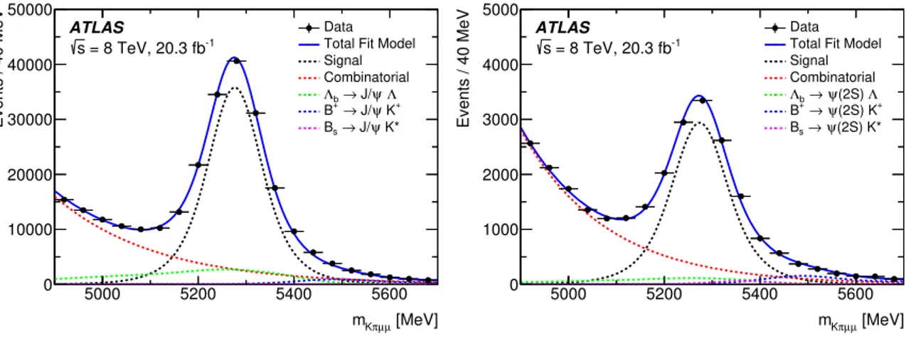
[MeV] µ µ π K m 5000 5200 5400 5600 Events / 40 MeV 0 10000 20000 30000 40000 50000 ATLAS -1 = 8 TeV, 20.3 fb s Data Total Fit Model Signal Combinatorial Λ ψ J/ → b Λ + K ψ J/ → + B K* ψ J/ → s B [MeV] µ µ π K m 5000 5200 5400 5600 Events / 40 MeV 0 1000 2000 3000 4000 5000 ATLAS -1 = 8 TeV, 20.3 fb s Data Total Fit Model Signal Combinatorial Λ (2S) ψ → b Λ + (2S) K ψ → + B (2S) K* ψ → s B

Figure 3. Fits to theKπµµ invariant mass distributions for the (left) K∗_{J/ψ and (right) K}∗_ψ(2S)

control region samples. The data are shown as points and the total fit model as the solid lines. The dashed lines represent (black) signal, (red) combinatorial background, (green) Λb background,

(blue)B+ _{background and (magenta)B}0

s background components.

they accumulate around 0.7 in | cos

θ

L

|. These are removed from the data sample when

estimating systematic uncertainties, as described in section

7

.

5.3

K

∗

cc control sample fits

The mass distribution obtained from the simulated samples for

K

∗

_{cc decays, respectively}

as

q

2

_{∈ [8, 11] and [12, 15] GeV}

2

_{, and the signal mode, in different bins of}

_q

2

_{, are found to}

be consistent with each other. Values of

m

0

and

ξ for B

0_d

→ K

∗

J/ψ and B

_d0

→ K

∗

ψ(2S)

events are used for the signal pdf and extracted from fits to the data. An extended unbinned

maximum-likelihood fit is performed in the two

K

∗

cc control region samples. There are

three exclusive backgrounds included: Λ

b

→ Λcc, B

+

→ K

+

cc and B

0s

→ K

∗

cc. The

K

∗

_{cc pdf has the same form as the signal model, combinatorial background is described}

by an exponential distribution, and double and triple Gaussian pdfs determined from MC

simulated events are used to describe the exclusive background contributions. A systematic

uncertainty is evaluated by allowing for 0, 1, 2 and 3 exclusive background components.

The control sample fit projections for the variant of the fit including all three exclusive

backgrounds can be found in figure

3

. The impact of the used exclusive background model

on the peak position and scale factor of the signal pdf is negligible. From these fits the

statistical and systematic uncertainties in the values of

m

0

and

ξ are extracted for the B

_d0

component in order to be used in the

B

0

d

→ K

∗

µ

+

µ

−

fits. From the

J/ψ control data

it is determined that the values for the nuisance parameters describing the signal model

pdf in the

Kπµµ mass are m

0

= 5276.6 ± 0.3 ± 0.4 MeV and ξ = 1.210 ± 0.004 ± 0.002,

where the uncertainties are statistical and systematic, respectively. The

ψ(2S) sample

yields compatible results albeit with larger uncertainties. These results are similar to those

obtained from the MC simulated samples, and the numbers derived from the

K

∗

J/ψ data

are used for the signal region fits.

JHEP10(2018)047

5.4

Fitting procedure and validation

A two-step fit process is performed for the different signal bins in

q

2

_{. The first step is a fit}

to the

Kπµ

+

_µ

−

_{invariant mass distribution, using the event-by-event uncertainty in the}

reconstructed mass as a conditional variable. For this fit, the parameters

m

0

and

ξ are

fixed to the values obtained from fits to data control samples as described in section

5.3

. A

second step adds the (transformed) cos

θ

K

, cos

θ

L

and

φ variables to the likelihood in order

to extract

F

L

and the

S parameters along with the values for the nuisance parameters

related to the combinatorial background shapes. Some nuisance parameters, namely

m

0

,

ξ, signal and background yields, and the exponential shape parameter for the background

mass pdf, are fixed to the results obtained from the first step.

The fit procedure is validated using ensembles of simulated pseudo-experiments

gen-erated with the

F

L

and

S parameters corresponding to those obtained from the data. The

purpose of these experiments is to measure the intrinsic fit bias resulting from the

likeli-hood estimator used to extract signal parameters. These ensembles are also used to check

that the uncertainties extracted from the fit are consistent with expectations. Ensembles

of simulated pseudo-experiments are performed in which signal MC events are injected into

samples of background events generated from the likelihood. The signal yield determined

from the first step in the fit process is found to be unbiased. The angular parameters

ex-tracted from the nominal fits have biases with magnitudes ranging between 0.01 and 0.04,

depending on the fit variation and

q

2

_{bin. A similar procedure is used to estimate the effect}

of neglecting

S-wave contamination in the data sample. Neglecting the S-wave component

in the fit model results in a bias between 0.00 and 0.02 in the angular parameters.

Simi-larly, neglecting exclusive background contributions from Λ

b

,

B

+

and

B

s0

decays that peak

in

m

Kπµµ

near the

B

_d0

mass results in a bias of less than 0.01 on the angular parameters.

All these effects are included in the systematic uncertainties described in section

7

. The

P

(0)

_{parameters are obtained using the fit results and covariance matrices from the second}

fit along with equations (

2.2

)–(

2.5

).

6

Results

The event yields obtained from the fits are summarised in table

1

where only statistical

un-certainties are reported. Figures

4

through

9

show for the different

q

2

_{bins the distributions}

of the variables used in the fit for the

S

5

folding scheme (corresponding to the

transfor-mation of equation (

5.3

)) with the total, signal and background fitted pdfs superimposed.

Similar sets of distributions are obtained for the three other folding schemes:

S

4

,

S

7

and

S

8

. The results of the angular fits to the data in terms of the

S

i

and

P

_j(0)

can be found

in tables

2

and

3

. Statistical and systematic uncertainties are quoted in the tables. The

distributions of

F

L

and the

S

i

parameters as a function of

q

2

are shown in figure

10

and

those for

P

_j(0)

are shown in figure

11

. The correlations between

F

L

and the

S

i

parameters

and between

F

L

and the

P

j(0)

are given in appendix

A

.

JHEP10(2018)047

q

2

_[GeV

2

_]

_n

signal

n

background

[0.04, 2.0]

128 ± 22

122 ± 22

[2.0, 4.0]

106 ± 23

113 ± 23

[4.0, 6.0]

114 ± 24

204 ± 26

[0.04, 4.0]

236 ± 31

233 ± 32

[1.1, 6.0]

275 ± 35

363 ± 36

[0.04, 6.0]

342 ± 39

445 ± 40

Table 1. The values of fitted signal, nsignal, and background, nbackground, yields obtained for

different bins inq2_{. The uncertainties indicated are statistical.}

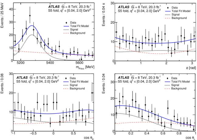
[MeV] µ µ π K m 5200 5400 5600 Events / 25 MeV 0 10 20 30 40 -1 = 8 TeV, 20.3 fb s ATLAS 2 [0.04, 2.0] GeV ∈ 2 S5 fold, q Data Total Fit Model Signal Background [rad] φ 0 1 2 3 π Events / 0.04 0 10 20 30 -1 = 8 TeV, 20.3 fb s ATLAS 2 [0.04, 2.0] GeV ∈ 2 S5 fold, q Data Total Fit Model Signal Background K θ cos 1 − −0.5 0 0.5 1 Events / 0.08 0 10 20 30 -1 = 8 TeV, 20.3 fb s ATLAS 2 [0.04, 2.0] GeV ∈ 2 S5 fold, q Data Total Fit Model Signal Background L θ cos 0 0.2 0.4 0.6 0.8 1 Events / 0.04 0 10 20 30 -1 = 8 TeV, 20.3 fb s ATLAS 2 [0.04, 2.0] GeV ∈ 2 S5 fold, q Data Total Fit Model Signal Background

Figure 4. The distributions of (top left)mKπµµ, (top right)φ, (bottom left) cos θK, and (bottom

right) cosθL obtained for q2 ∈ [0.04, 2.0] GeV2. The (blue) solid line is a projection of the total

pdf, the (red) dot-dashed line represents the background, and the (black) dashed line represents the signal component. These plots are obtained from a fit using theS5 folding scheme.

JHEP10(2018)047

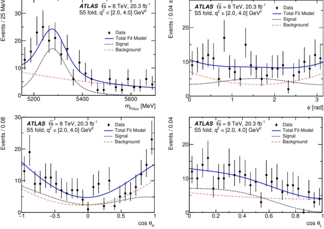
[MeV] µ µ π K m 5200 5400 5600 Events / 25 MeV 0 10 20 30 -1 = 8 TeV, 20.3 fb s ATLAS 2 [2.0, 4.0] GeV ∈ 2 S5 fold, q Data Total Fit Model Signal Background [rad] φ 0 1 2 3 π Events / 0.04 0 10 20 -1 = 8 TeV, 20.3 fb s ATLAS 2 [2.0, 4.0] GeV ∈ 2 S5 fold, q Data Total Fit Model Signal Background K θ cos 1 − −0.5 0 0.5 1 Events / 0.08 0 10 20 30 -1 = 8 TeV, 20.3 fb s ATLAS 2 [2.0, 4.0] GeV ∈ 2 S5 fold, q Data Total Fit Model Signal Background L θ cos 0 0.2 0.4 0.6 0.8 1 Events / 0.04 0 10 20 -1 = 8 TeV, 20.3 fb s ATLAS 2 [2.0, 4.0] GeV ∈ 2 S5 fold, q Data Total Fit Model Signal Background

Figure 5. The distributions of (top left)mKπµµ, (top right)φ, (bottom left) cos θK, and (bottom

right) cosθL obtained forq2∈ [2.0, 4.0] GeV2. The (blue) solid line is a projection of the total pdf,

the (red) dot-dashed line represents the background, and the (black) dashed line represents the signal component. These plots are obtained from a fit using the S5folding scheme.

JHEP10(2018)047

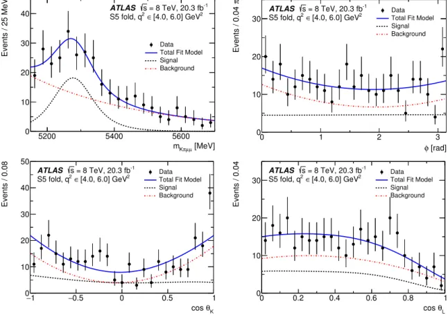
[MeV] µ µ π K m 5200 5400 5600 Events / 25 MeV 0 10 20 30 40 -1 = 8 TeV, 20.3 fb s ATLAS 2 [4.0, 6.0] GeV ∈ 2 S5 fold, q Data Total Fit Model Signal Background [rad] φ 0 1 2 3 π Events / 0.04 0 10 20 30 -1 = 8 TeV, 20.3 fb s ATLAS 2 [4.0, 6.0] GeV ∈ 2 S5 fold, q Data Total Fit Model Signal Background K θ cos 1 − −0.5 0 0.5 1 Events / 0.08 0 10 20 30 40 50 -1 = 8 TeV, 20.3 fb s ATLAS 2 [4.0, 6.0] GeV ∈ 2 S5 fold, q Data Total Fit Model Signal Background L θ cos 0 0.2 0.4 0.6 0.8 1 Events / 0.04 0 10 20 30 -1 = 8 TeV, 20.3 fb s ATLAS 2 [4.0, 6.0] GeV ∈ 2 S5 fold, q Data Total Fit Model Signal Background

Figure 6. The distributions of (top left)mKπµµ, (top right)φ, (bottom left) cos θK, and (bottom

right) cosθL obtained forq2∈ [4.0, 6.0] GeV2. The (blue) solid line is a projection of the total pdf,

the (red) dot-dashed line represents the background, and the (black) dashed line represents the signal component. These plots are obtained from a fit using the S5folding scheme.

JHEP10(2018)047

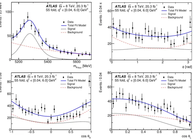
[MeV] µ µ π K m 5200 5400 5600 Events / 25 MeV 0 20 40 60 -1 = 8 TeV, 20.3 fb s ATLAS 2 [0.04, 4.0] GeV ∈ 2 S5 fold, q Data Total Fit Model Signal Background [rad] φ 0 1 2 3 π Events / 0.04 0 10 20 30 40 -1 = 8 TeV, 20.3 fb s ATLAS 2 [0.04, 4.0] GeV ∈ 2 S5 fold, q Data Total Fit Model Signal Background K θ cos 1 − −0.5 0 0.5 1 Events / 0.08 0 20 40 -1 = 8 TeV, 20.3 fb s ATLAS 2 [0.04, 4.0] GeV ∈ 2 S5 fold, q Data Total Fit Model Signal Background L θ cos 0 0.2 0.4 0.6 0.8 1 Events / 0.04 0 20 40 -1 = 8 TeV, 20.3 fb s ATLAS 2 [0.04, 4.0] GeV ∈ 2 S5 fold, q Data Total Fit Model Signal Background

Figure 7. The distributions of (top left)mKπµµ, (top right)φ, (bottom left) cos θK, and (bottom

right) cosθL obtained for q2 ∈ [0.04, 4.0] GeV2. The (blue) solid line is a projection of the total

pdf, the (red) dot-dashed line represents the background, and the (black) dashed line represents the signal component. These plots are obtained from a fit using theS5 folding scheme.

JHEP10(2018)047

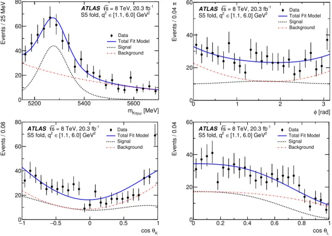
[MeV] µ µ π K m 5200 5400 5600 Events / 25 MeV 0 20 40 60 80 -1 = 8 TeV, 20.3 fb s ATLAS 2 [1.1, 6.0] GeV ∈ 2 S5 fold, q Data Total Fit Model Signal Background [rad] φ 0 1 2 3 π Events / 0.04 0 20 40 60 -1 = 8 TeV, 20.3 fb s ATLAS 2 [1.1, 6.0] GeV ∈ 2 S5 fold, q Data Total Fit Model Signal Background K θ cos 1 − −_{0.5 0 0.5 1} Events / 0.08 0 20 40 60 80 -1 = 8 TeV, 20.3 fb s ATLAS 2 [1.1, 6.0] GeV ∈ 2 S5 fold, q Data Total Fit Model Signal Background L θ cos 0 0.2 0.4 0.6 0.8 1 Events / 0.04 0 20 40 60 -1 = 8 TeV, 20.3 fb s ATLAS 2 [1.1, 6.0] GeV ∈ 2 S5 fold, q Data Total Fit Model Signal Background

Figure 8. The distributions of (top left)mKπµµ, (top right)φ, (bottom left) cos θK, and (bottom

right) cosθL obtained forq2∈ [1.1, 6.0] GeV2. The (blue) solid line is a projection of the total pdf,

the (red) dot-dashed line represents the background, and the (black) dashed line represents the signal component. These plots are obtained from a fit using the S5folding scheme.

JHEP10(2018)047

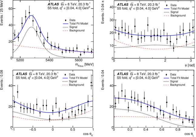
[MeV] µ µ π K m 5200 5400 5600 Events / 25 MeV 0 50 100 -1 = 8 TeV, 20.3 fb s ATLAS 2 [0.04, 6.0] GeV ∈ 2 S5 fold, q Data Total Fit Model Signal Background [rad] φ 0 1 2 3 π Events / 0.04 0 20 40 60 -1 = 8 TeV, 20.3 fb s ATLAS 2 [0.04, 6.0] GeV ∈ 2 S5 fold, q Data Total Fit Model Signal Background K θ cos 1 − −0.5 0 0.5 1 Events / 0.08 0 20 40 60 80 -1 = 8 TeV, 20.3 fb s ATLAS 2 [0.04, 6.0] GeV ∈ 2 S5 fold, q Data Total Fit Model Signal Background L θ cos 0 0.2 0.4 0.6 0.8 1 Events / 0.04 0 20 40 60 80 -1 = 8 TeV, 20.3 fb s ATLAS 2 [0.04, 6.0] GeV ∈ 2 S5 fold, q Data Total Fit Model Signal Background

Figure 9. The distributions of (top left)mKπµµ, (top right)φ, (bottom left) cos θK, and (bottom

right) cosθL obtained for q2 ∈ [0.04, 6.0] GeV2. The (blue) solid line is a projection of the total

pdf, the (red) dot-dashed line represents the background, and the (black) dashed line represents the signal component. These plots are obtained from a fit using theS5 folding scheme.

JHEP10(2018)047

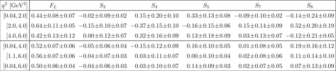
q2_[GeV2_{] F} L S3 S4 S5 S7 S8 [0.04, 2.0] 0.44±0.08±0.07 −0.02±0.09±0.02 0.15±0.20±0.10 0.33±0.13±0.08 −0.09±0.10±0.02 −0.14±0.24±0.09 [2.0, 4.0] 0.64±0.11±0.05 −0.15±0.10±0.07 −0.37±0.15±0.10 −0.16±0.15±0.06 0.15±0.14±0.09 0.52±0.20±0.19 [4.0, 6.0] 0.42±0.13±0.12 0.00±0.12±0.07 0.32±0.16±0.09 0.13±0.18±0.09 0.03±0.13±0.07 −0.12±0.21±0.05 [0.04, 4.0] 0.52±0.07±0.06 −0.05±0.06±0.04 −0.15±0.12±0.09 0.16±0.10±0.05 0.01±0.08±0.05 0.19±0.16±0.12 [1.1, 6.0] 0.56±0.07±0.06 −0.04±0.07±0.03 0.03±0.11±0.07 0.00±0.10±0.04 0.02±0.08±0.06 0.11±0.14±0.10 [0.04, 6.0] 0.50±0.06±0.04 −0.04±0.06±0.03 0.03±0.10±0.07 0.14±0.09±0.03 0.02±0.07±0.05 0.07±0.13±0.09

Table 2. The values ofFL, andS3,S4,S5,S7 andS8parameters obtained for different bins inq2.

The uncertainties indicated are statistical and systematic, respectively.

q2_[GeV2_{] P} 1 P 0 4 P 0 5 P 0 6 P 0 8 [0.04, 2.0] −0.05±0.30±0.08 0.31±0.40±0.20 0.67±0.26±0.16 −0.18±0.21±0.04 −0.29±0.48±0.18 [2.0, 4.0] −0.78±0.51±0.34 −0.76±0.31±0.21 −0.33±0.31±0.13 0.31±0.28±0.19 1.07±0.41±0.39 [4.0, 6.0] 0.14±0.43±0.26 0.64±0.33±0.18 0.26±0.35±0.18 0.06±0.27±0.13 −0.24±0.42±0.09 [0.04, 4.0] −0.22±0.26±0.16 −0.30±0.24±0.17 0.32±0.21±0.11 0.01±0.17±0.10 0.38±0.33±0.24 [1.1, 6.0] −0.17±0.31±0.13 0.05±0.22±0.14 0.01±0.21±0.08 0.03±0.17±0.12 0.23±0.28±0.20 [0.04, 6.0] −0.15±0.23±0.10 0.05±0.20±0.14 0.27±0.19±0.06 0.03±0.15±0.10 0.14±0.27±0.17

Table 3. The values of P1, P40, P50, P60 andP80 parameters obtained for different bins in q2. The

uncertainties indicated are statistical and systematic, respectively.

7

Systematic uncertainties

Systematic uncertainties in the parameter values obtained from the angular analysis come

from several sources. The methods for determining these uncertainties are based either

on a comparison of nominal and modified fit results, or on observed fit biases in modified

pseudo-experiments. The systematic uncertainties are symmetrised. The most significant

ones are described in the following, in decreasing order of importance.

• A systematic uncertainty is assigned for the combinatorial Kπ (fake K

∗

) background

peaking at cos

θ

K

values around 1.0 obtained by comparing results of the nominal fit

to that where data above cos

θ

K

= 0.9 are excluded from the fit.

• A systematic uncertainty is derived to account for background arising from partially

reconstructed

B → D

0

_/D

+

_/D

+

s

X decays, that manifest in an accumulation of events

at | cos

θ

L

| values around 0.7. Two-track or three-track combinations are formed from

the signal candidate tracks, and are reconstructed assuming the pion or kaon mass

hypothesis. A veto is then applied for events in which a track combination has a mass

in a window of 30 MeV around the

D

0

_,

_D

+

_or

_D

+

s

meson mass. Similarly, a veto is

implemented to reject

B

+

_{→ K}

+

_µ

+

_µ

−

_and

_B

+

_{→ π}

+

_µ

+

_µ

−

_{events that pass the event}

selection. Here

B

+

_{candidates are reconstructed from one of the hadrons from the}

_K

∗

candidate and the muons in the signal candidate. Signal candidates that have a

three-track mass within 50 MeV of the

B

+

_{mass are excluded from the fit. A few percent}

of signal events are removed when applying these vetoes, with a corresponding effect

on the acceptance distributions. The fit results obtained from the data samples with

JHEP10(2018)047

vetoes applied are compared to those obtained from the nominal fit and the change

in each result is taken as the systematic uncertainty from these backgrounds. This

systematic uncertainty dominates the measurement of

F

L

at higher values of

q

2

.

• The combinatorial background pdf shape has an uncertainty arising from the choice

of the model. For the mass distribution it is assumed that an exponential function

model is adequate; however, for the angular variables the data are re-fitted using

third-order Chebychev polynomials. The change from the nominal result is taken as

the uncertainty from this source.

• The acceptance function is assumed to factorise into three separate components, for

cos

θ

K

, cos

θ

L

and

φ. To validate this assumption, the signal simulated events are

fitted with the acceptance function obtained from that same MC sample. Differences

in the fit results from expectation are small and taken as the uncertainty resulting

from this assumption.

• A systematic uncertainty is assigned for the angular pdf model for the background

by comparing the nominal result to that with a reduced fit range of

m

Kπµµ

∈

[5200, 5700] MeV, in particular to account for possible residues of the partially

re-constructed

B-decays.

• A correction is applied to the data by shifting the track p

T

according to the

uncer-tainties arising from biases in rapidity and momentum scale. The change in results

obtained is ascribed to the uncertainty in the ID alignment and knowledge of the

magnetic field.

• The maximum-likelihood estimator used is intrinsically biased. Ensembles of MC

simulated events are used in order to ascertain the bias in the extracted values of the

parameters of interest. The bias is assigned as a systematic uncertainty.

• The p

T

spectrum of

B

_d0

candidates observed in data is not accurately reproduced by

the MC simulation. This difference in the kinematics results in a slight modification

of the acceptance functions. This is accounted for by reweighting signal MC simulated

events to resemble the

p

T

spectrum found in data. The change in fitted parameter

values obtained due to the reweighting is taken as the systematic uncertainty resulting

from this difference.

• The signal decay mode is resonant K

∗

_{→ Kπ decay, but scalar contributions from}

non-resonant

Kπ transitions may also exist. The LHCb Collaboration reported an

S-wave contribution at the level of 5% of the signal [

4

,

30

]. Ensembles of MC simulated

events are fitted with 5% of the signal being drawn from an

S-wave sample of events

and the remaining 95% from signal. The observed change in fit bias is assigned as

the systematic uncertainty from this source. Any variation in

S-wave content as a

function of

q

2

_{would not significantly affect the results reported here.}

JHEP10(2018)047

• The values of the nuisance parameters of the fit model obtained from MC control

samples and fits to the data mass distribution have associated uncertainties. These

parameters include

m

0

,

ξ, the signal and background yields, the shape parameter of

the combinatorial background mass distribution, and the parameters of the signal

acceptance functions. The uncertainty in the value of each of these parameters is

varied independently in order to assess the effect on parameters of interest. This

source of uncertainty has a small effect on the measurements reported here.

• Background from exclusive modes peaking in m

Kπµµ

is neglected in the nominal

fit.

This may affect the fitted results and is accounted for by computing the

fit bias obtained when embedding MC simulated samples of Λ

b

→ Λ(1520)µ

+

µ

−

,

Λ

b

→ pK

−

µ

+

µ

−

,

B

+

→ K

(∗)+

µ

+

µ

−

and

B

s0

→ φµ

+

µ

−

into ensembles of

pseudo-data generated from the fit model containing only combinatorial background and

sig-nal components. The change in fit bias observed when adding exclusive backgrounds

is taken as the systematic error arising from neglecting those modes in the fit.

• The difference from nominal results obtained when fitting the B

0

d

signal MC events

with the acceptance function for

B

0

d

is taken as an upper limit of the systematic error

resulting from event migration due to mistagging the

B

0

d

flavour.

• The parameters S

5

and

S

8

, as well as the respective

P

_j(0)

parameters are affected by

dilution and thus have a multiplicative scaling applied to them. This dilution factor

depends on the kinematics of the

K

∗

decay and has a systematic uncertainty

associ-ated with it. The effect of data/MC differences in the

p

T

spectrum of

B

d0

candidates

on the mistag probability was studied and found to be negligible. The uncertainty due

to the limited number of MC events is used to compute the statistical uncertainty of

ω

and

ω. Studies of MC simulated events indicate that there is no significant difference

between the mistag probability for

B

0

d

and

B

0d

events and the analysis assumes that

the average mistag probability provides an adequate description of this effect. The

magnitude of the mistag probability difference, |ω − ω|, is included as a systematic

uncertainty resulting from this assumption.

The total systematic uncertainties of the fitted

S

i

and

P

_j(0)

parameter values are presented

in tables

2

and

3

, where the dominant contributions for

F

L

come from the modelling of

the angular distributions of the combinatorial background and the partially reconstructed

decays peaking in cos

θ

K

and cos

θ

L

. These contributions and in addition also ID alignment

and magnetic field calibration affect

S

3

(P

1

). The largest systematic uncertainty

contribu-tion to

S

3

(P

1

) comes from partially reconstructed decays entering the signal region. This

also affects the measurement of

S

5

(P

50

) and

S

7

(P

60

). The partially reconstructed decays

peaking in cos

θ

L

affect the measurement of

S

4

(P

40

) and

S

8

(P

80

), whereas the fake

K

∗

back-ground in cos

θ

K

affects

S

4

(P

40

),

S

5

(P

50

), and

S

8

(P

80

). The parameterization of the signal

acceptance is another significant systematic uncertainty source for

S

4

(P

40

). The systematic

uncertainties are smaller than the statistical uncertainties for all parameters measured.

JHEP10(2018)047

0 2 4 6 8 10 ] 2 [GeV 2 q 0 0.2 0.4 0.6 0.8 1 1.2 1.4 1.6 1.8 L F Data CFFMPSV fit theory DHMV theory JC ATLAS _{s = 8 TeV, 20.3 fb}-1 0 2 4 6 8 10 ] 2 [GeV 2 q 0.4 − 0.2 − 0 0.2 0.4 0.6 0.8 3 S Data CFFMPSV fit theory DHMV ATLAS s = 8 TeV, 20.3 fb-1 0 2 4 6 8 10 ] 2 [GeV 2 q 0.6 − 0.4 − 0.2 − 0 0.2 0.4 0.6 0.8 4 S Data CFFMPSV fit theory DHMV ATLAS _{s = 8 TeV, 20.3 fb}-1 0 2 4 6 8 10 ] 2 [GeV 2 q 0.6 − 0.4 − 0.2 − 0 0.2 0.4 0.6 0.8 5 S Data CFFMPSV fit theory DHMV ATLAS s = 8 TeV, 20.3 fb-1 0 2 4 6 8 10 ] 2 [GeV 2 q 0.4 − 0.2 − 0 0.2 0.4 0.6 0.8 7 S Data CFFMPSV fit theory DHMV ATLAS _{s = 8 TeV, 20.3 fb}-1 0 2 4 6 8 10 ] 2 [GeV 2 q 0.4 − 0.2 − 0 0.2 0.4 0.6 0.8 8 S Data CFFMPSV fit theory DHMV ATLAS s = 8 TeV, 20.3 fb-1

Figure 10. The measured values of FL, S3, S4, S5, S7, S8 compared with predictions from the

theoretical calculations discussed in the text (section 8). Statistical and total uncertainties are shown for the data, i.e. the inner mark indicates the statistical uncertainty and the total error bar the total uncertainty.

8

Comparison with theoretical computations

The results of theoretical approaches of Ciuchini et al. (CFFMPSV) [

31

], Descotes-Genon

et al. (DHMV) [

32

], and J¨

ager and Camalich (JC) [

33

,

34

] are shown in figure

10

for the

S

parameters, and in figure

11

for the

P

(0)

_{parameters, along with the results presented here.}

4

4_{This result uses the experimental convention of equations (2.2)–(2.5) following the LHCb Collaboration’s}

notation in ref. [3]. In the DHMV calculation, a different convention is used as explained by equation (16) in ref. [15].

JHEP10(2018)047

0 2 4 6 8 10 ] 2 [GeV 2 q 2 − 1.5 − 1 − 0.5 − 0 0.5 1 1.5 2 1 P Data theory DHMV theory JC ATLAS _{s = 8 TeV, 20.3 fb}-1 0 2 4 6 8 10 ] 2 [GeV 2 q 2 − 1.5 − 1 − 0.5 − 0 0.5 1 1.5 2 4 P' Data theory DHMV theory JC ATLAS _{s = 8 TeV, 20.3 fb}-1 0 2 4 6 8 10 ] 2 [GeV 2 q 1 − 0.5 − 0 0.5 1 1.5 2 5 P' Data CFFMPSV fit theory DHMV theory JC ATLAS _{s = 8 TeV, 20.3 fb}-1 0 2 4 6 8 10 ] 2 [GeV 2 q 1 − 0.5 − 0 0.5 1 1.5 2 6 P' Data theory DHMV theory JC ATLAS _{s = 8 TeV, 20.3 fb}-1 0 2 4 6 8 10 ] 2 [GeV 2 q 1 − 0.5 − 0 0.5 1 1.5 2 8 P' Data theory DHMV theory JC ATLAS _{s = 8 TeV, 20.3 fb}-1

Figure 11. The measured values of P1, P40, P50, P60, P80 compared with predictions from the

theoretical calculations discussed in the text (section 8). Statistical and total uncertainties are shown for the data, i.e. the inner mark indicates the statistical uncertainty and the total error bar the total uncertainty.

QCD factorisation is used by DHMV and JC, where the latter focus on the impact

of long-distance corrections using a helicity amplitude approach. The CFFMPSV group

takes a different approach, using the QCD factorisation framework to perform compatibility

checks of the LHCb data with theoretical predictions. This approach also allows

informa-tion from a given experimentally measured parameter of interest to be excluded in order to

make a fit-based prediction of the expected value of that parameter from the rest of the data.

JHEP10(2018)047

With the exception of the

P

0

4

and

P

50

measurements in

q

2

∈ [4.0, 6.0] GeV

2

and

P

80

in

q

2

_{∈ [2.0, 4.0] GeV}

2

_{there is good agreement between theory and measurement. The}

_P

0

4

and

P

0

5

parameters have statistical correlation of 0.37 in the

q

2

∈ [4.0, 6.0] GeV

2

bin. The

ob-served deviation from the SM prediction of

P

₄0

and

P

₅0

is for both parameters approximately

2.7 standard deviations (local) away from the calculation of DHMV for this bin. The

devi-ations are less significant for the other calculation and the fit approach. All measurements

are found to be within three standard deviations of the range covered by the different

pre-dictions. Hence, including experimental and theoretical uncertainties, the measurements

presented here are found to agree with the predicted SM contributions to this decay.

9

Conclusion

The results of an angular analysis of the rare decay

B

0

d

→ K

∗

_µ

+

_µ

−

_{are presented. This}

flavour-changing neutral current process is sensitive to potential new-physics contributions.

The

B

0

d

→ K

∗

µ

+

µ

−

analysis presented here uses a total of 20.3 fb

−1

_of

√

s = 8 TeV pp

col-lision data collected by the ATLAS experiment at the LHC in 2012. An extended unbinned

maximum-likelihood fit of the angular distribution of the signal decay is performed in order

to extract the parameters

F

L

,

S

i

and

P

j(0)

in six bins of

q

2

. Three of these bins overlap in

order to report results in ranges compatible with other experiments and phenomenology

studies. All measurements are found to be within three standard deviation of the range

covered by the different predictions. The results are also compatible with the results of the

LHCb, CMS and Belle collaborations.

Acknowledgments

We thank CERN for the very successful operation of the LHC, as well as the support staff

from our institutions without whom ATLAS could not be operated efficiently.

We acknowledge the support of ANPCyT, Argentina; YerPhI, Armenia; ARC,

Aus-tralia; BMWFW and FWF, Austria; ANAS, Azerbaijan; SSTC, Belarus; CNPq and

FAPESP, Brazil; NSERC, NRC and CFI, Canada; CERN; CONICYT, Chile; CAS, MOST

and NSFC, China; COLCIENCIAS, Colombia; MSMT CR, MPO CR and VSC CR,

Czech Republic; DNRF and DNSRC, Denmark; IN2P3-CNRS, CEA-DRF/IRFU, France;

SRNSFG, Georgia; BMBF, HGF, and MPG, Germany; GSRT, Greece; RGC, Hong Kong

SAR, China; ISF, I-CORE and Benoziyo Center, Israel; INFN, Italy; MEXT and JSPS,

Japan; CNRST, Morocco; NWO, Netherlands; RCN, Norway; MNiSW and NCN, Poland;

FCT, Portugal; MNE/IFA, Romania; MES of Russia and NRC KI, Russian Federation;

JINR; MESTD, Serbia; MSSR, Slovakia; ARRS and MIZˇ

S, Slovenia; DST/NRF, South

Africa; MINECO, Spain; SRC and Wallenberg Foundation, Sweden; SERI, SNSF and

Cantons of Bern and Geneva, Switzerland; MOST, Taiwan; TAEK, Turkey; STFC, United

Kingdom; DOE and NSF, United States of America. In addition, individual groups and

members have received support from BCKDF, the Canada Council, CANARIE, CRC,

Compute Canada, FQRNT, and the Ontario Innovation Trust, Canada; EPLANET, ERC,

ERDF, FP7, Horizon 2020 and Marie Sk lodowska-Curie Actions, European Union;

In-vestissements d’Avenir Labex and Idex, ANR, R´

egion Auvergne and Fondation Partager