• Sonuç bulunamadı

An application of supplier evaluation process

N/A
N/A
Protected

Academic year: 2021

Share "An application of supplier evaluation process"

Copied!
86
0
0

Yükleniyor.... (view fulltext now)

Tam metin

(1)

AN APPLICATION OF SUPPLIER EVALUATION

PROCESS

Yiğit GÖLDELİ

Thesis Advisor: Asst.Prof.Dr.Adalet ÖNER

Department of Industrial Engineering

Bornova – IZMIR 2014

(2)
(3)

YAŞAR UNIVERSITY

GRADUATE SCHOOL OF NATURAL AND APPLIED SCIENCES

AN APPLICATION OF SUPPLIER EVALUATION

PROCESS

Yiğit GÖLDELİ

Thesis Advisor: Asst.Prof.Dr.Adalet ÖNER

Department of Industrial Engineering

Bornova – IZMIR 2014

(4)
(5)

iii

This study titled “AN APPLICATION OF SUPPLIER EVALUATION PROCESS” and presented as MSc Thesis by Yiğit GÖLDELİ has been evaluated in compliance with the relevant provisions of Y.U. Graduate Education and Training Regulation and Y.U. Institute of Science Education and Training Direction and jury members written below have decided for the defense of this thesis and it has been declared by consensus / majority of votes that he candidate has succeeded in thesis defense examination dated July,2014.

Jury Members : Signature:

Head :……… ……….

Rapporteur Member : ………. ……….

(6)
(7)

v

ÖZET

TEDARİKÇİ DEĞERLENDİRME SÜREÇLERİNE

YÖNELİK BİR UYGULAMA

GÖLDELİ, Yiğit

Yüksek Lisans Tezi, Endüstri Mühendisliği Programı Tez Danışmanı: Yrd. Doç. Dr. Adalet ÖNER

Haziran 2014, 62 sayfa

Bu çalışmada farklı tedarikçi değerlendirme yöntemleri incelenerek, farklı sektörlerde hizmet veren iki firmada uygulaması gösterilmiştir. Bu amaçla en çok kullanılan Analitik Hiyerarşi Süreci (AHP) ve TOPSIS yöntemleri seçilmiştir. Tedarikçilerin değerlendirilmesi için belirlenen kriterlerin farklı sektörler için nasıl farklılaştıkları irdelenmiştir. Birlikte çalışılan firmalar için üçer adet alternatif tedarikçi belirlenmiştir Her iki yöntemle de tedarikçilerin değerlendirilmesi yapılmış, öncelikleri belirlenmiş ve elde edilen sonuçlar karşılaştırılmıştır.

Anahtar Kelimeler: Analitik Hiyerarşi Süreci (AHP), TOPSIS, tedarikçi seçimi

(8)
(9)

vii

ABSTRACT

AN APPLICATION OF SUPPLIER EVALUATION

PROCESS

GÖLDELİ, Yiğit

MSc in Industrial Engineering Supervisor: Asst. Prof. Dr. Adalet ÖNER

June 2014, 62 Pages

This study concerns with the application of supplier evaluation process for purchasing departments of two different companies operating in different industrial sectors in Izmir. Evaluating suppliers is usually a complex multi-criteria decision making problem in which decision maker needs to evaluate the alternatives under both qualitative and quantitative criteria. There are many approaches to solve this problem however there is no proven best method. In this study, Analytical Hierarchy Process (AHP) and TOPSIS methods have been used for evaluating and ranking the suppliers. The details of evaluating process have been presented. The outcomes has been classified, compared and discussed. It is interesting to observe how different companies use some common and disjoint criteria depending on their profile and the industries in which they operate. Criteria sets used in other studies in literature have also been studied and compared.

Keywords: Analytical Hierarchy Process (AHP), TOPSIS, supplier selection

(10)
(11)

ix

ACKNOWLEDGEMENTS

I would like to acknowledge the advice and guidance of Asst. Prof. Adalet Öner for his support and help.

I also thank the experts of the Küçükbay A.Ş. and Timsan Traktör for their supports, guidance and suggestions, especially Yasir KALAYCI, Kadriye GÜRBÜZ, Sedat ŞİPŞAK for their supports, guidance and suggestions and encouragements.

I would like to give special thanks to my wife, my family and my dearest friends for supporting and encouraging me. Especially without their encouragement, I would not have finished this project.

(12)
(13)

xi

TEXT OF OATH

I declare and honestly confirm that my study titled “AN APPLICATION OF SUPPLIER EVALUATION PROCESS”, and presented as Master’s Thesis has been written without applying to any assistance inconsistent with scientific ethics and traditions and all sources I have benefited from are listed in bibliography and I have benefited from these sources by means of making references.

30 / 06/ 2014

(14)

TABLE OF CONTENTS Page ÖZET……… v ABSTRACT………. vii ACKNOWLEDGEMENTS………. ix TEXT OF OATH………. xi

INDEX OF FIGURES………. xiv

INDEX OF TABLES……….. xx

INDEX OF SYMBOLS AND ABBREVIATIONS……….……….. xxi

1. INTRODUCTION……… 1

2. STATEMENT OF THE PROBLEM…………..………..………... 2

3. LITERATURE REVIEW………. 4

4. ANALYTIC HIERARCHY PROCESS…………..………. 8

4.1 Basic Principles of AHP Methodology……….. 10

4.2 Test of Consistency……… 11

5. TOPSIS………..……….. 16

6. APPLICATIONS OF THE MODELS IN SUPPLIER SELECTION………. 18

6.1 AHP Model………..……….………. 19

6.2 The Details of the Comparison Criteria………...………. 21

6.2.1 Quality………...……….………. 21

6.2.2 Compliance with Standards……..……...……….... 21

(15)

xiii

TABLE OF CONTENTS (continued)

6.2.4 Geographical Position….………...………... 22

6.2.5 After Sales Services………...………... 22

6.2.6 Payment Term……….……...………... 23

6.2.7 Price……… 23

6.2.8 Lead Time……..………... 24

6.2.9 Production Capacity……… 24

6.2.10 Flexibility of Delivery Time………. 24

6.2.11 R&D Power………... 25

6.3 Evaluation of the Hierarchy of Timsan Company…..……….….… 25

6.4 Evaluation of the Hierarchy of Küçükbay Company……… 36

6.5 TOPSIS Model……….. 47

6.6 Evaluation of the Hierarchy of Timsan Company…..……….….… 48

6.7 Evaluation of the Hierarchy of Küçükbay Company……… 50

7. RESULTS AND DISCUSSION…..………..………. 52

(16)

INDEX OF FIGURE

FIGURE PAGE

4.1 Sample Hierarchy Structure ………. 9

6.1 Hierarchical Model of Timsan…………....………..……... 20

6.2 Hierarchical Model of Küçükbay………...………..……... 20

6.3 Synthesis of Model for Timsan Company……… 35

(17)

xv

INDEX OF TABLES

TABLE PAGE

3.1 List of Studies for Supplier Evaluation………... 6

4.2 Preference scale of pairwise comparisons………... 11

4.3 Sample Pairwise Comparison Matrix……….………... 11

4.4 The Complete Sample Pairwise Comparison Matrix……… 12

4.5 Column Totals of pairwise Comparison Matrix…....……… 13

4.6 Normalized Matrix………..………..……… 13

4.7 Sample Eigenvector………..………..………..……… 14

4.8 Random Consistency Indices ……...…………..………..……… 14

6.1 Comparisons of Criteria Used in AHP Model 19 6.2 Distances of Supplier from the Companies……… 22

6.3 Response Times of Suppliers……… 22

6.4 Payment Terms……….……. 23

6.5 Prices Offered by Suppliers………...…… 23

6.6 Lead Times of Suppliers………...………. 24

(18)

INDEX OF TABLES (continued)

TABLE PAGE

6.8 Pairwise Comparison Matrix for Main Criteria….….………..…….. 26

6.9 Normalized Matrix of Main Criteria………... 26

6.10 Weights of Main Criteria ……….………... 27

6.11 Pairwise Comparisons w.r.t. “Quality” …..………....….…... 27

6.12 Normalized Matrix w.r.t. “Quality”……….…………....……... 27

6.13 Local Priorities of Alternatives w.r.t. “Quality”………. 28

6.14 Pairwise Comparisons w.r.t. “Compliance with Standards”………... 28

6.15 Normalized Matrix w.r.t. “Compliance with Standards”……… 28

6.16 Local Priorities of Alternatives w.r.t. “Compliance with Standards”. 29 6.17 Pairwise Comparisons w.r.t. “Reliability of Supplier”…………... 29

6.18 Normalized Matrix w.r.t. “Reliability of Supplier”……… 29

6.19 Local Priorities of Alternatives w.r.t. “Reliability of Supplier”…… 30

6.20 Pairwise Comparisons w.r.t. “Geo. Position”……… 30

6.21 Normalized Matrix w.r.t. “Geo. Position”………. 30

(19)

xvii

INDEX OF TABLES (continued)

TABLE PAGE

6.23 Pairwise Comparisons w.r.t. “After Sales Services”……….. 31

6.24 Normalized Matrix w.r.t. “After Sales Services”………... 31

6.25 Local Priorities of Alternatives w.r.t. “After Sales Services”……… 32

6.26 Pairwise Comparisons w.r.t. “Price”……….. 32

6.27 Normalized Matrix w.r.t. “Price”………... 32

6.28 Local Priorities of Alternatives w.r.t. “Price”……… 33

6.29 Pairwise Comparisons w.r.t. “Payment Term”……….. 33

6.30 Normalized Matrix w.r.t. “Payment Term”……… 33

6.31 Local Priorities of Alternatives w.r.t. “Payment Term”………. 33

6.32 Local Priorities of Alternatives for Timsan………... 34

6.33 Pairwise Comparison Matrix for Main Criteria………. 36

6.34 Normalized Matrix of Main Criteria……….. 36

6.35 Weights of Main Criteria……… 37

(20)

INDEX OF TABLES (continued)

TABLE PAGE

6.37 Normalized Matrix w.r.t. “Quality”………... 37

6.38 Local Priorities of Alternatives w.r.t. “Quality”……….. 38

6.39 Pairwise Comparisons w.r.t. “Price”……… 38

6.40 Normalized Matrix w.r.t. “Price”………. 38

6.41 Local Priorities of Alternatives w.r.t. “Price”……….. 39

6.42 Pairwise Comparisons w.r.t. “Lead Time”………... 39

6.43 Normalized Matrix w.r.t. “Lead Time”……..……….. 39

6.44 Local Priorities of Alternatives w.r.t. “Lead Time”……..…………... 40

6.45 Pairwise Comparisons w.r.t. “After Sales Services”……… 40

6.46 Normalized Matrix w.r.t. “After Sales Services”………. 40

6.47 Local Priorities of Alternatives w.r.t. “After Sales Services”……… 41

6.48 Pairwise Comparisons w.r.t. “Production Capacity”………. 41

6.49 Normalized Matrix w.r.t. “Production Capacity”……….. 41

6.50 Local Priorities of Alternatives w.r.t. “Production Capacity”……… 42

(21)

xix

INDEX OF TABLES (continued)

TABLE PAGE

6.52 Normalized Matrix w.r.t. “Flexibility of Delivery Time”………….. 42

6.53 Local Priorities of Alternatives w.r.t. “Flexibility of DeliveryTime” 43 6.54 Pairwise Comparisons w.r.t. “R&D Power”……….. 43

6.55 Normalized Matrix w.r.t. “R&D Power”………... 43

6.56 Local Priorities of Alternatives w.r.t. “R&D Power”……… 44

6.57 Pairwise Comparisons w.r.t. “Geo. Position”……… 44

6.58 Normalized Matrix w.r.t. “Geo. Position”………. 44

6.59 Local Priorities of Alternatives w.r.t. “Geo. Position”………... 45

6.60 Local Priorities of Alternatives for Küçükbay Calculations...……... 45

6.61 Pairwise Comparison Matrices for Timsan Company……….. 48

6.62 Weights of Criteria for Timsan Company ………... 48

6.63 Normalization of Criteria for Timsan Company ……….. 49

6.64 Weighted Normalization of Criteria for Timsan Company …….. 49

(22)

INDEX OF TABLES (continued)

TABLE PAGE

6.66 Closeness the Ideal Solution for Timsan Company ……….…. 50

6.67 Pairwise Comparisons Matrices for Küçükbay Company………. 50

6.68 Weights of Criteria for Küçükbay Company ………. 50

6.69 Normalization of Criteria for Küçükbay Company ……….. 51

6.70 Weighted Normalization of Criteria for Küçükbay Company …….. 51

6.71 Ideal and Negative Solutions for Küçükbay Company ………. 51

6.72 Closeness the Ideal Solution for Küçükbay Company ……….…. 51

7.1 Comparison Table for Timsan………. 52

7.2 Comparison Table for Küçükbay………. 52

(23)

xxi

INDEX OF SYMBOLS AND ABBREVIATIONS

SYMBOLS

n Number of compared components

A Pairwise Comparison Matrix

𝑎𝑎𝑖𝑖𝑖𝑖 Elements in Pairwise Comparison Matrix

B Normalized Matrix

𝑏𝑏𝑖𝑖𝑖𝑖 Elements in Normalized Matrix

wi Eigenvector

λmax Maximum Eigenvalue

CI Consistency Index

CR Consistency Ratio

RI Random Consistency Index

w Preference (weight) vector

C The columns are the eigenvectors of the pairwise comparisons of the alternatives

(24)

INDEX OF SYMBOLS AND ABBREVIATIONS (continued)

ABBREVIATION

AHP Analytic Hierarchy Process

TOPSIS The Technique for Order of Preference by Similarity to Ideal Solution

(25)

1 1. INTRODUCTION

In most industries, the cost of raw materials and component parts has the greatest share in the overall cost of a product. For this reason, purchasing strategy and procedures have a critical role to control the input costs. One of the main functions of purchasing department is to evaluate the suppliers in a systematic procedure and choosing the appropriate ones.

Identifying the best suppliers should meet the goal of receiving the right quantity on the right time with the right cost. Choosing the right suppliers will decrease company’s purchasing cost, increase customer satisfaction and improve the power of competition.

Supplier evaluation is usually a complex multi-criteria decision making problem involving both qualitative and quantitative elements. There is no proven best method and companies deploy a variety of different approaches.

This study deals with evaluating and ranking of suppliers. Two analysis tools are considered in the study. The first one is the “Analytical Hierarchy Process (AHP)” and the other one is the “Technique for Order of Preference by Similarity to Ideal Solution (TOPSIS)” method. Both of the methods are well known and used frequently in multiple criteria decision making problems.

Two companies from different sectors have been chosen to show the application of supplier evaluation methods. It is interesting to observe how they use some common and disjoint criteria depending on the industries in which they operate.

The rest of the study is organized as follows. Information about the companies and statement of problem is given in the next chapter. Chapter three includes literature survey. Chapter four and five are devoted to basic brief descriptions of AHP and TOPSIS methodologies respectively. Applications of AHP and TOPSIS methods for supplier selection are given in chapter 6. All numerical details and computations are presented in that chapter. Chapter seven includes results, comparisons of outcomes and discussion.

(26)

Two different companies from different sectors have been selected for application of supplier evaluation process. The “Küçükbay” company is in food industry and produces cooking oil including sunflower, corn, canola and soya oils. It offers its products to consumers with ‘Orkide Oil’ brand at home and with ‘Orkide’ and ‘Vera’ brands abroad. It has a wide sales network comprised of many dealers in 81 cities in 7 regions of Turkey. Its products are exported to more than 90 countries worldwide. Recently the company increases its efforts to make Orkide a worldwide brand.

The sector leader with a daily refined oil capacity of 1000 tons, Küçükbay meets 35% of Turkey’s annual cooking oil consumption. Operating in an area of approximately 30,000 square meters, Küçükbay and its 250 employees adopt four main principles that make ‘Orkide’ and ‘Vera’ national and international brands: quality, advanced technology, product variety and superior capacity.

The “Küçükbay” company purchases the containers of the products in general such as different types glass bottles, bottle caps, labeling material, tin boxes or sheets of tin.

The “Timsan” company, founded in 2009, produces towing tractors used only at airports. Due to the nature of the sector, the company uses make-to-order policy instead of mass production. The products of the company include small-sized tractors towing luggage trailers, mid-small-sized tractors towing airport cargo trailers & small airplanes, and push-back vehicles towing airplanes.

The company currently exports 85% of its products. The goal of the company for the following years is to increase domestic sales since ground services of national air carriers purchase same products from foreign companies. Purchases of national carriers may even reach to a level as high as production capacity of “Timsan” company.

(27)

3

“Timsan” company purchases a wide variety of materials to use in different stages of its production. It purchases engines, gears, differential gears, metal sheet, wiper motors etc. The quality of purchased parts is as important as price since “Timsan” provides 2-year warranty period

The goal of this study is to evaluate potential suppliers and determining relative priorities of them in order to help the purchasing departments of the companies. It is a multi-criteria decision making problem involving both qualitative and quantitative elements. AHP and TOPSIS methods will be used for evaluating the suppliers. The details of the evaluation processes will be given for both methods for each company. The outcomes will then be compared and discussed.

(28)

In industries that are concerned with large scale production, the cost of the raw materials and components parts is equal up to 70% of product cost. In such a case, the purchasing department can play a key role in cost reduction, and supplier selection is one of the most important functions of purchasing management (Ho et al, 2010), and therefore, using an appropriate method for this purpose is a critical issue. Supplier evaluation has been shown to be multiple criteria decision making (MCDM) problem (Weber et al 1991). There are many methodologies and approaches for solving supplier evaluation problem. However AHP and TOPSIS are the most common methods which have been used for this purpose.

Analytic Hierarchy Process (AHP) is a special technique, used in multi-criteria decision making problems. It is a technique that provides with a systematic structure for evaluating and ranking the alternatives under various criteria.

AHP is proven to be a useful tool especially when decision maker needs to evaluate the alternatives under both qualitative and quantitative criteria. AHP method was introduced by Saaty (1977, 1980), and it is used in a widespread area of applications. The typical application areas are reviewed below.

Evaluating and ranking of projects is one of the application areas in which AHP is used as the primary decision tool. There may be many projects developed in a company. Since the resources are scarce, those projects should be ranked in order to decide the priorities. The projects usually have different aspects and originated from different departments of the company. Therefore they have to be evaluated under both qualitative and quantitative criteria such as contribution to the strategic goals, costs, benefits, urgency, risks etc. For example Pehlivanlı (2005) developed an AHP model to how to evaluate and deciding the priorities of the projects in Turkish Army. Some other applications are explained in Al Khalil (2002) and Muralidhar et al (1990).

(29)

5

Strategic planning deals with developing effective strategies for the companies. AHP may be used for evaluating different potential strategy alternatives as seen in Zaim et al (2012).

In cost-benefit analysis, AHP method is used to evaluate alternatives. Evaluation criteria consist of cost, characteristics, technical specifications, risks, safety and flexibility. Tuleda et al (2006) developed an AHP model to conduct cost-benefit analysis in a transport project.

Wickramasinghe and Takano (2009) studied a systematic approach for strategic marketing planning of a tourism revival project. He used a combination of SWOT analysis and Analytic Hierarchy Process methodology.

Curry and Moutinho (1992) propose an AHP model which is implemented in a computer application for comparative decisions for environmental issues in tourism management.

Finally AHP is also used in evaluating and ranking of suppliers. Selecting appropriate supplier is a multi-criteria decision making problem that considers objectives such as cost, quality, delivery time etc. There are many studies that explain how AHP can be used for supplier evaluation such as Akarte (2011), Chan and Chan (2004), Kahraman et al (2003), Çebi and Bayraktar (2003) andBruno et al (2012). All studies have the same objective of determining priorities of suppliers. However comparison criteria are somehow different in each study although there are some common ones. Table 3.1 shows a list of studies for supplier evaluation (Supçiller and Çapraz, 2011). Table also shows the different criteria used for supplier evaluation. The table is updated and improved in this study.

The technique for order preference by similarity to Ideal Solution (TOPSIS) was first developed by Yoon and Hwang (1981). TOPSIS has been a favorable technique for solving multi criteria problems. This is mainly for two reasons; the first one is that its concept is reasonable and easy to understand. The second reason is that it requires less computational efforts, and therefore can be applied easily in comparison with other MCDM methods, like AHP.

(30)

Nr Researcher Year Methods

Criterion

Quality Price After Sales Service

Delivery

Time Flexibility Technology Performance Supplier

Compliance with Standards

Geographical

Position Payment Term Risk

Relationship (Reliability of Supplier) Creativity (R&D Power) Supplier Profile Facility 1 Nydick and Hill 1992 AHP 1 1 1 1 2 Ghodsypur and O'Brien 1998 AHP 1 1 1 3 Yahya and Kingsman 1999 AHP 1 1 1 1 1 4 Dağdeviren and Eren 2001 AHP 1 1 1 1 5 Tam and Tummala 2001 AHP 1 1 6 Chan and Chan 2004 AHP 1 1 1 1 1 1 7 Wang et al 2004 AHP 1 1 1 1 8 Liu and Hai 2005 AHP 1 1 1 1 1 9 Yang and Chen 2006 AHP 1 1 1 1 1 1 1 10 Paksoy and Güleş 2006 AHP 1 1 1 1 1 11 Chan and Kumar 2007 Fuzzy AHP 1 1 1 1 1 12 Xia and Wu 2007 AHP 1 1 1 13 Stevenson 2007 AHP 1 1 1 1 1 14 Jharkharia and Shankar 2007 AHP + TOPSIS 1 1 15 Seçme and Özdemir 2008 Fuzzy AHP 1 1 1 1 1 16 Chan et al 2008 Fuzzy AHP 1 1 1 1 17 Ecer and Küçük 2008 AHP 1 1 1 1 18 Mendoza et al 2008 AHP 1 1 1 1 1 19 Wang et al. 2009 Fuzzy TOPSIS 1 1 1 20 Boran et al 2009 Fuzzy TOPSIS 1 1 1 1 21 Ku et al 2010 Fuzzy AHP 1 1 1 1 22 Bagheri and Tarokh 2010 AHP + Fuzzy TOPSIS

23 Özdemir 2010 AHP 1 1 1 1 1 1 1 1

24 Fazlollahtabar et al. 2011 AHP + TOPSIS 1 1 1 1 1 25 Ishizaka et al 2012 AHP 1 1 1 1

26 Bruno et al 2012 AHP 1 1 1 1

27 Chengjing Jounio 2013 AHP 1 1 1 1 28 Kim et al 2013 AHP 1 1 1 1 29 Tayyar and Arslan 2013 AHP + VIKOR 1 1 1 1 30 Ömürbek et al 2013 AHP 1 1 1 1 1 31 Ömürbek and Kınay 2013 TOPSIS 1 1 1 1

(31)

7

TOPSIS is based on the concept that the optimal alternative should have the shortest distance from the positive ideal solution (PIS) and the farthest distance from the negative ideal solution (NIS). TOPSIS method is a powerful decision making process which help people to set priorities on parameters that are to be considered by reducing complex decision to a series of one to one comparisons, thereby synthesizing the result. (C. Elanchezian et al, 2010 ) The studies that uses TOPSIS are Jharkharia and Shankar (2007), Wang et al (2009), Baron et al (2009), Bagheri and Tarokh (2010), Fazlollahtaber et al (2011), Ömürbek and Kınay (2013).

(32)

Analytic Hierarchy Process (AHP) is a technique which is used in multi-criteria decision problems to make the best choice between alternatives. AHP is useful tool especially when decision maker needs to evaluate the alternatives under both qualitative and quantitative criteria. Essence of the technique depends on pairwise comparisons to choose the best alternative.

According to Saaty (1994) the analytic hierarchy process is an effective system for solving complex decision making problems, and may assist the decision maker to set priorities and make the best decision.

The analytic hierarchy process method consists of three levels of hierarchy. The first level of hierarchy is the objective of the decision making, the second level of hierarchy is how each of the existing criteria contributes to the achievement, and the last level of hierarchy is to find out how each of the alternatives contributes to each of the criteria. Main structure of hierarchy model is shown in Figure 4.1. Taylor (2002) explains that the steps of decision making process using by the method are as follows:

• Determine the objective, main-criteria, sub-criteria, alternatives and construction of the hierarchy.

• Make pairwise comparisons of criteria

• Make pairwise comparisons of alternatives for each criteria • Calculation of priority vectors

• Calculate and check consistency ratio • Analysis of the AHP scores

(33)

9

Figure 4.1 Sample Hierarchy Structure

GOAL OF THE PROBLEM MAIN- CRITERIA SUB- CRITERIA ALTERNATIVES 9

(34)

Saaty (1994) states that AHP method consists of three basic principles which are as defined below:

• Decomposition

The decision problem is decomposed into some hierarchical components such as the objective of the problem, performance criteria including sub-criteria and the solution alternatives. Those components are combined to form a hierarchical tree structure.

• Comparative Judgement

The essence of AHP method is to make pairwise comparisons between the components of the hierarchical structure. Those comparisons help us to evaluate the relative importance of the components. A special evaluation method is used through pairwise comparisons. The results can be observed in the form of Pairwise Comparison Matrices.

• Synthesis of Priority

Each pairwise comparison matrix is used to determine local priorities. The global priorities are then acquired by synthesizing those local priorities that is called weights.

A ratio-scale form is used in pairwise comparisons. It imposes subjective evaluation between the components. Actually it asks the decision maker to decide the relative importance of the components and express the subjective judgement in a numerical format. It shows the degree of preference of a component over the other one. Those values are then stored in the pairwise comparison matrix. The ratio-scale is limited in a range between 1–9. The standard preference scale of pairwise comparison is explained in Table 4.2.

(35)

11

Table 4.2 Preference scale of pairwise comparisons Intensity of

Importance Definition Explanation

1 Equally Preferred Two components contribute equally to the objective

3 Moderate Preferred Experience and judgement slightly favors one component over another

5 Strong Preferred Experience and judgement strongly favors one component over another

7 Very Strong

Preferred

An component is favored very strongly over another, its dominance demonstrated in practice 9 Extreme Preferred The evidence favoring one component over another

is of the highest possible order of affirmation

2,4,6,8

Intermediate values between two adjacent scale values

-

4.2 Test of Consistency

AHP method checks the consistency of the pairwise comparisons in order to get a reliable solution. Inconsistency arises in different situations. Consider that there are 3 components (A, B and C) are the subject of pairwise comparisons. If the decision maker makes a pairwise comparison between A and B and decides A is moderately preferred over B by using preference intensity 3. Furthermore, consider he/she decides preference intensity is 2 when B compared to C and preference intensity is 2 when A compared to C. The decisions are then showed in a pairwise comparison matrix as shown below.

Table 4.3 Sample Pairwise Comparison Matrix

COMPONENT A B C

A 1 3 2

B 1 2

(36)

missing elements are filled with appropriate reciprocal values. Resulting comparison matrix is shown in Table 4.4

Table 4.4 The Complete Sample Pairwise Comparison Matrix

COMPONENT A B C

A 1 3 2

B 1/3 1 2

C 1/2 1/2 1

There is some inconsistency in Table 4.4 since the preference intensity should be 6 when A compared to C based on the two previous comparisons (A vs. B and B vs. C). Let 𝑎𝑎𝑖𝑖𝑖𝑖 denote the elements in the pairwise comparison matrix. This matrix is consistent when the following equality is true for each i, j, and k

𝑎𝑎𝑖𝑖𝑖𝑖 𝑎𝑎𝑖𝑖𝑖𝑖 = 𝑎𝑎𝑖𝑖𝑖𝑖 ∀ 𝑖𝑖, 𝑗𝑗 𝑎𝑎𝑎𝑎𝑎𝑎 𝑘𝑘 (1)

This formula is an expression of the transitivity of preferences. The inconsistency in Table 4.4 may be revealed for i=1, j=2 and k=3. Although consistency requires 𝑎𝑎13 𝑎𝑎32= 𝑎𝑎12 , the values in that table don’t meet the requirement 2 ∗1

2≠ 3. If 𝑎𝑎13 = 6 instead of 2, then consistency would be

provided.

However, the consistency check is made in a different way in practice. Taylor (2002) defines a special procedure and the term “consistency index” that is used for consistency check for each pairwise comparison matrix.

n : number of compared components

A : pairwise comparison matrix (for example shown in Table 4.4) 𝑎𝑎𝑖𝑖𝑖𝑖 : elements in matrix A ( i= 1,..,n; j=1,..,n)

(37)

13

The comparison matrix A is “normalized” in order to get matrix B. Normalization process is conducted simply by dividing each element of 𝑎𝑎𝑖𝑖𝑖𝑖 by the column totals. Therefore 𝑏𝑏𝑖𝑖𝑖𝑖 , the elements of matrix B can be found as follows: 𝑏𝑏𝑖𝑖𝑖𝑖 = 𝑎𝑎𝑖𝑖𝑖𝑖𝑎𝑎

𝑖𝑖𝑖𝑖 𝑛𝑛

𝑖𝑖=1 (2)

The details of establishing matrix B is illustrated in the following two tables.

Table 4.5 Column Totals of Pairwise Comparison Matrix

COMPONENT A B C A 1 3 2 B 1/3 1 2 C 1/2 1/2 1 SUM OF THE COLUMN 1 + 1 3 + 1 2 3 + 1 + 1 2 2 + 2 + 1

Table 4.6 Normalized Matrix

COMPONENT A B C A 1 1 + 13 +12 0,67 0,40 B 0,18 0,22 0,40 C 0,27 0,11 0,20

Then, the eigenvector w : (w1, w2, …. , wn) of the normalized matrix B, and

maximum eigenvalue, 𝜆𝜆𝑚𝑚𝑚𝑚𝑚𝑚, is defined as follows:

𝑤𝑤𝑖𝑖 = ∑ 𝑏𝑏𝑖𝑖𝑖𝑖 𝑛𝑛 𝑖𝑖=1 𝑎𝑎 (3) 𝜆𝜆𝑚𝑚𝑚𝑚𝑚𝑚 = 𝑎𝑎 �1 (𝑨𝑨𝑨𝑨)𝑤𝑤 𝑖𝑖 𝑖𝑖 𝑛𝑛 𝑖𝑖=1 (4)

(38)

Table 4.7 Sample Eigenvector COMPONENT wi A 0,55 + 0,18 + 0,27 3 B 0,27 C 0,19

𝜆𝜆

𝑚𝑚𝑚𝑚𝑚𝑚

=

13

(

𝐴𝐴𝐴𝐴𝐴𝐴11

+

𝐴𝐴𝐴𝐴𝐴𝐴22

+

𝐴𝐴𝐴𝐴𝐴𝐴33

) =

3.13

The Consistency Index (CI) is defined and numerical calculation is made as follows:

𝐶𝐶𝐶𝐶 =𝜆𝜆𝑚𝑚𝑎𝑎𝑚𝑚−𝑎𝑎

𝑎𝑎−1 (5)

𝐶𝐶𝐶𝐶 =3,13 − 33 − 1 = 0,068

After that, Consistency Ratio (CR) formula is defined as follows:

𝐶𝐶𝐶𝐶 =𝐶𝐶𝐶𝐶𝑅𝑅𝐶𝐶 where RI is Random Consistency Index (6)

Random Consistency Index (RI) values are calculated as a function of the number of components, n. The methodology of calculation is given in Saaty (1994). Those values are usually presented in tables as shown in Table 4.8.

Table 4.8 Random Consistency Indices

n 1 2 3 4 5 6 7 8 9 10

RI 0 0 0,52 0,89 1,11 1,25 1,35 1,40 1,45 1,49

Numerical calculation is shown below based on the sample above;

(39)

15

The test of consistency is completed when the CR is numerically calculated. The decision of consistency is made depending on the numerical value of CR.

If CR ≥ 10%, achieved data is inconsistent

If CR < 10%, achieved data is consistent

If we are to evaluate the consistency of the sample comparison matrix given in Table 4.3, we need to decide that comparisons are not consistent since CR value is 0.13 ≥ 0.10.

(40)

SIMILARITY TO IDEAL SOLUTION (TOPSIS)

The TOPSIS is a multi-criteria decision analysis method, which was originally developed by Hwang and Yoon in 1981 with further developments by Yoon in 1987, and Hwang, Lai and Liu in 1993.

TOPSIS is based on the concept that the chosen alternative should have the shortest geometric distance from the positive ideal solution and the longest geometric distance from the negative ideal solution. It is a method of compensatory aggregation that compares a set of alternatives by identifying weights for each criterion, normalizing scores for each criterion and calculating the geometric distance between each alternative and the ideal alternative, which is the best score in each criterion. An assumption of TOPSIS is that the criteria are monotonically increasing or decreasing. Normalization is usually required as the parameters or criteria are often of incongruous dimensions in multi-criteria problems. Compensatory methods such as TOPSIS allow trade-offs between criteria, where a poor result in one criterion can be negated by a good result in another criterion. This provides a more realistic form of modelling than non-compensatory methods, which include or exclude alternative solutions based on hard cut-offs. The TOPSIS process is carried out as follows:

Step 1

Construct normalized decision matrix. This step transforms various attribute dimensions into non-dimensional attributes, which allows comparisons across criteria. Normalize scores or data as follows:

𝑟𝑟𝑖𝑖𝑖𝑖 = 𝑚𝑚𝑖𝑖𝑖𝑖/(∑ 𝑚𝑚𝑖𝑖𝑖𝑖2) For 𝑖𝑖 = 1, … , 𝑚𝑚 , 𝑗𝑗 = 1, … , 𝑎𝑎

Step 2

Construct the weighted normalized decision matrix. Assume we have a set of weights for each criteria, 𝑤𝑤𝑖𝑖 , ∀𝑗𝑗 = 1, … , 𝑎𝑎. Multiply each column of the normalized decision matrix by its associated weight. The elements of the new matrix are defined as 𝑤𝑤𝑖𝑖𝑖𝑖 = 𝑤𝑤𝑖𝑖𝑟𝑟𝑖𝑖𝑖𝑖

(41)

17

Step 3

Determine the ideal and negative ideal solutions. Ideal solution

𝐴𝐴∗ = {𝑣𝑣

1∗, … , 𝑣𝑣∗𝑛𝑛} , where 𝑣𝑣𝑖𝑖∗ = �𝑚𝑚𝑎𝑎𝑚𝑚 (𝑣𝑣𝑖𝑖𝑖𝑖)𝑖𝑖𝑖𝑖 𝑗𝑗 ∈ 𝐽𝐽 ; min (𝑣𝑣𝑖𝑖𝑖𝑖)𝑖𝑖𝑖𝑖 𝑗𝑗 ∈ 𝐽𝐽′�

Negative ideal solution 𝐴𝐴′= {𝑣𝑣

1′, … , 𝑣𝑣𝑛𝑛′} , where 𝑣𝑣′= �𝑚𝑚𝑖𝑖𝑎𝑎 (𝑣𝑣𝑖𝑖𝑖𝑖)𝑖𝑖𝑖𝑖 𝑗𝑗 ∈ 𝐽𝐽 ; max (𝑣𝑣𝑖𝑖𝑖𝑖)𝑖𝑖𝑖𝑖 𝑗𝑗 ∈ 𝐽𝐽′�

Step 4

Calculate the separation measures for each alternative. The separation from the ideal alternative is:

𝑆𝑆𝑖𝑖 ∗ = [∑(𝑣𝑣𝑖𝑖∗− 𝑣𝑣𝑖𝑖𝑖𝑖)2]1/2 For 𝑖𝑖 = 1, … , 𝑚𝑚

Similarly, the separation from the negative ideal alternative is: 𝑆𝑆𝑖𝑖 = [∑(𝑣𝑣

𝑖𝑖′− 𝑣𝑣𝑖𝑖𝑖𝑖)2]1/2 For 𝑖𝑖 = 1, … , 𝑚𝑚

Step 5

Calculate the relative closeness to the ideal solution 𝐶𝐶𝑖𝑖

𝐶𝐶𝑖𝑖∗ = 𝑆𝑆𝑖𝑖′/(𝑆𝑆𝑖𝑖∗+ 𝑆𝑆𝑖𝑖′), 0 < 𝐶𝐶𝑖𝑖∗ < 1 Select the option with 𝐶𝐶𝑖𝑖∗closest to 1.

Step 6

(42)

SELECTION

The goal of this study is to evaluate suppliers and determining relative priorities in order to help purchasing department for deciding which supplier should be preferred. AHP and TOPSIS methods will be used for evaluating the suppliers. These two methods may be used in a combined way as in the following directions (Ghosh, 2011). In this procedure, first AHP is performed and the outcomes are fed into TOPSIS method. Steps of combined evaluation method are listed as follows:

AHP:

Step 1: Selection of Experts

Step 2: Identify the Attributes/Criteria Step 3: Identify the Alternatives Step 4: Design the Hierarchy

Step 5: Establish the pair-wise comparison of the criteria Step 6: Calculate the Eigen value and Eigen vector Step 7: Perform the consistency test

Step 8: Compute the weights of the criteria

Step 9: Establish the pair-wise comparison of the alternatives with respect to each criteria

Step 10: Calculate the Eigen value and Eigen vector for each of them Step 11: Perform the Consistency Test

Step 12: Compute the weights of the Alternatives for each Criteria

Step 13: Calculate the geometric mean of the weights calculated by experts

Step 14: Calculate the Eigen value and Eigen vector Step 15: Perform the Consistency Tests

Step 16: Compute the overall weights of the alternatives TOPSIS:

Step 17: Start TOPSIS procedure using weights calculated using AHP Step 18: Calculate negative and positive ideal solutions & separation measures

(43)

19 6.1 AHP Model

Generally, there are three main components in AHP hierarchy. They are: the goal of the model, comparison criteria and the alternatives to be ranked. Two distinct models are developed for each company.

The goals of the models for both companies are defined as “Selection of the Best Supplier”. Since both companies purchase a wide variety of materials, suppliers are grouped in accordance with the material groups. For “Küçükbay” company, suppliers of tin boxes are considered only, whereas spare part suppliers are considered in “Timsan” company. Three alternative suppliers are determined for both companies and they are defined as “A”, “B” and “C” to mask the real names of suppliers.

The comparison criteria of the models are decided by decision makers comprised of experts from purchasing department and consultants in each company. Table 6.1 shows the comparison criteria in both models.

Table 6.1 Comparisons of Criteria Used in AHP Model

The structures of the hierarchies are shown below in Figure 6.1 and Figure 6.2.

Criteria Criterion 1 Criterion 2 Criterion 3 Criterion 4 Company

Timsan Quality Price After Sales

Services

Geographical Position

Küçükbay Quality Price After Sales

Services

Geographical Position

Criteria

Criterion 5 Criterion 6 Criterion 7 Criterion 8

Company Timsan Compliance with Standards Reliability of Supplies Payment Term Küçükbay Production

Capacity Lead Time

Flexibility of Delivery

Time

(44)

Figure 6.1 Hierarchical Model of Timsan

(45)

21 6.2 The Details of Comparison Criteria

In this section, the details of the comparison criteria will be presented. Each criterion will be explained in detail and justified why it is included in the model.

6.2.1 Quality

The quality criterion is always included in supplier evaluation. Quality defines the perception of satisfaction about the characteristics of a material that determine whether it meets the implied requirements.

The alternative suppliers are evaluated using subjective judgments considering specifications and requirements of the product. Pairwise comparisons made by experts of companies. An alternative gets higher priority as the quality increases.

6.2.2 Compliance with Standards

The Compliance with Standards criterion is selected to be considered in supplier evaluation. Standards are a system to identify, develop, acquire, evaluate, disseminate, and provide access to applicable standards, codes, regulations, and laws. This criterion is about how the suppliers comply with relevant standards of the industry in which they operate. Alternative suppliers are evaluated using subjective judgments considering specifications and requirements of the product. This criterion is used only for Timsan Company whereas it is not considered in Küçükbay. Pairwise comparisons made by experts of the company. An alternative gets higher priorities as its grade increases in “compliance with standards”.

6.2.3 Reliability of Supplier

The “reliability of supplier” criterion is another factor for purchasing department. Reliable supplier is described who deliver the right goods or services on time. Bigger suppliers are generally accepted as reliable because they have enough resources and systems in place to make sure that they can still deliver if anything goes wrong. Reliability of alternative suppliers is evaluated using

(46)

increases.

6.2.4 Geographical Position

“Geographical position” another factor is selected to be considered in supplier evaluation since it has impacts on delivery lead time, transportation, and logistics costs. Some organizations require their suppliers to be located within a certain distance from their facilities. The distances of suppliers from the companies are given in the following table. Since this criterion consists of numerical values, we don’t need to make subjective comparisons. An alternative is more preferable if its distance is less than the other alternative.

Table 6.2 Distances of Suppliers from the Companies

Geographical

Position A B C

Timsan 100 km 150 km 90 km

Küçükbay 100 km 120 km 70 km

6.2.5 After Sales Services

The “After Sales Services” is also a factor in supplier selection. Suppliers must be able to back up their products by providing good services when needed. For example, when product information or warranty service is needed, suppliers must respond on a timely basis. This criterion defines the response time of supplier when the products need to be replaced or some information is required. The numerical values for response time of suppliers are given in the following table. Since this criterion consists of numerical values, we don’t need to make subjective comparisons.

Table 6.3 Response Times of Suppliers

Response

Time A B C

Timsan 10 days 14 days 8 days

(47)

23 6.2.6 Payment Term

The “Payment Term” is a one of the factors to be considered in supplier selection. It defines the conveniences provided by the supplier such as deferred payment and longer maturity periods. This criterion is used only for Timsan Company whereas it is not considered in Küçükbay. Since this criterion consists of numerical values, we don’t need to make subjective comparisons. Therefore an alternative gets higher priority as the payment term increases. . The numerical values for payment terms of suppliers are given in the following table.

Table 6.4 Payment Terms

Payment

Term A B C

Timsan 30 days 45 days 90 days

6.2.7 Price

The price criterion is one of the factors in evaluating and ranking of alternatives. Unit prices are known for each supplier. Since price criterion consists of numerical values, we don’t need to make subjective comparisons. The model takes the numerical values and uses them directly in the synthesis. An alternative is preferred over the other one if its price is lower. The degree of preference changes depending on the difference of the prices. Therefore an alternative gets higher priority as its price decreases. The prices given by suppliers are presented in the following table however the entries are modified in order to maintain information security of the companies.

Table 6.5 Prices Offered by Suppliers

Price A B C

Timsan 1,5 $ 2 $ 3 $

(48)

The Lead Time is another factor in supplier selection. It is better to have a shorter lead time since it is helpful when production plans of the company require quick alterations. This criterion is used only for Küçükbay Company whereas it is not considered in Timsan. Since lead time criterion consists of numerical values, we don’t need to make subjective comparisons.

Table 6.6 Lead Times of Suppliers

Lead Time A B C

Küçükbay 4 days 3 days 4 days

6.2.9 Production Capacity

The Production Capacity is another factor in supplier selection. This criterion is used only for Küçükbay company but not in Timsan. Since production capacities of suppliers are known, we don’t need to make subjective comparisons. A supplier is more preferable if it has higher production capacity.

Table 6.7 Production Capacities of Suppliers

Production Capacity A B C Küçükbay 400.000 units/day 600.000 units/day 250.000 units/day

6.2.10 Flexibility of Delivery Time

The Flexibility of Delivery Time is another factor in supplier selection. The supplier is expected to deliver the products in predetermined lots sizes at the time windows that are specified in the arrangement. Flexibility of delivery time defines the ability of the supplier to comply the delivery schedule. Alternative suppliers are evaluated using subjective judgments. This criterion is used only for Küçükbay Company but not considered in Timsan. Pairwise comparisons made

(49)

25

by experts of the company. The entries represent the geometric means of individual judgments.

6.2.11 R&D Power

The R&D Power is another factor in supplier selection. The supplier should produce the new products at the expected time that is specified in the arrangement. This criterion is used only for Küçükbay Company but not in Timsan. The alternative suppliers are evaluated using subjective judgments. Pairwise comparisons made by experts of the company. An alternative gets higher priorities its grade increases in “R&D power”.

6.3 Evaluation of the Hierarchy of Timsan Company

As stated before, the essence of AHP is pairwise comparisons. The synthesis of AHP model is then made by manipulating pairwise comparison matrices. The comparison matrices may have subjective judgments or some direct numerical values. All the subjective judgments are made by experts from purchasing department. The entries in comparison matrices represent the geometric means of individual judgments.

The synthesis or the overall outcome of the model is found in two stages. The local priorities of main criteria is calculated in the first stage. In the second stage, the local priorities of alternatives are found with respect to each main criteria and finally overall outcome is found using those local priorities.

The first stage starts with the comparisons at the first level which refer to pairwise comparisons of main criteria (see Table 6.8). The values represent subjective judgements.

(50)

MAIN CRITERIA Quality Compliance with Standards Reliability of Supplier Geographical Position After Sales Services Price Payment Term Quality 1,00 0,20 5,00 5,00 2,00 9,00 5,00 Compliance with Standards 5,00 1,00 3,00 7,00 3,00 9,00 9,00 Reliability of Supplier 0,20 0,33 1,00 2,00 2,00 3,00 2,00 Geographical Position 0,20 0,14 0,50 1,00 0,50 7,00 2,00 After Sales Services 0,50 0,33 0,50 2,00 1,00 5,00 3,00 Price 0,11 0,11 0,33 0,14 0,20 1,00 0,33 Payment Term 0,20 0,11 0,50 0,50 0,33 3,03 1,00 Sum 7,21 2,23 10,83 17,64 9,03 37,03 22,33

Pairwise comparison matrix is then normalized and consistency ratio is calculated as explained in section 4.2 and normalized matrix is presented in Table 6.9.

Table 6.9. Normalized Matrix of Main Criteria

MAIN CRITERIA Quality Compliance with Standards Reliability of Supplier Geographical Position After Sales Services Price Payment Term Quality 0,1387 0,0896 0,4615 0,2834 0,2214 0,2430 0,2239 Compliance with Standards 0,6934 0,4481 0,2769 0,3968 0,3321 0,2430 0,4030 Reliability of Supplier 0,0277 0,1494 0,0923 0,1134 0,2214 0,0810 0,0896 Geographical Position 0,0277 0,0640 0,0462 0,0567 0,0554 0,1890 0,0896 After Sales Services 0,0693 0,1494 0,0462 0,1134 0,1107 0,1350 0,1343 Price 0,0154 0,0498 0,0308 0,0081 0,0221 0,0270 0,0148 Payment Term 0,0277 0,0498 0,0462 0,0283 0,0369 0,0818 0,0448

Consistency Ratio (CR) of matrix =0,0839

The relative importance, or weights, or the local priorities of main criteria are then defined by the averages of each row in normalized matrix. These values are presented in Table 6.10.

(51)

27

Table 6.10 Weights of Main Criteria

WEIGHTS Quality 0,2374 Compliance with Standards 0,3990 Reliability of Supplier 0,1107 Geographical Position 0,0755 After Sales Services 0,1083 Price 0,0240 Payment Term 0,0451

In the second stage, the local priorities of alternatives should be calculated with respect to each main criteria. The first comparison of alternatives is done with respect to main criterion “Quality”. The comparison matrix is given below in Table 6.11. The comparison matrix includes subjective judgments.

Table 6.11 Pairwise Comparisons w.r.t. “Quality”

Quality A B C

A 1,000 2,000 3,000

B 0,500 1,000 0,750

C 0,667 1,333 1,000

Sum 2,167 4,333 3,250

Pairwise comparison matrix is then normalized and consistency ratio is calculated and presented in Table 6.12.

Table 6.12 Normalized Matrix w.r.t. “Quality”

Quality A B C

A 0,462 0,462 0,462

B 0,231 0,231 0,231

C 0,308 0,308 0,308

Consistency Ratio (CR) of matrix =0,00

The relative importance or the local priorities of alternatives w.r.t. “Quality” are then defined by the averages of each row in normalized matrix. These values are presented in Table 6.13.

(52)

The second comparison of alternatives is done with respect to main criterion “Compliance with Standards”. The comparison matrix is given below in Table 6.14. The comparison matrix includes subjective judgements.

Table 6.14 Pairwise Comparisons w.r.t. “Compliance with Standards”

Compliance with Standards A B C A 1,000 2,000/1,500 1,000/1,500 B 0,750 1,000 1,000/2,000 C 1,500 2,000 1,00 Sum 3,250 4,333 2,167

Pairwise comparison matrix is then normalized and consistency ratio is calculated and presented in Table 6.15.

Table 6.15 Normalized Matrix w.r.t. “Compliance with Standards”

Compliance with Standards A B C A 0,308 0,308 0,308 B 0,231 0,231 0,231 C 0,462 0,462 0,462

Consistency Ratio (CR) of matrix =0,00

The relative importance or the local priorities of alternatives w.r.t. “Compliance with Standards” are then defined by the averages of each row in normalized matrix. These values are presented in Table 6.16.

WEIGHTS

A 0,462

B 0,231

(53)

29

Table 6.16 Local Priorities of Alternatives w.r.t. “Compliance with Standards”

WEIGHTS

A 0,308

B 0,231

C 0,462

The third comparison of alternatives is done with respect to main criterion “Reliability of Supplier”. The comparison matrix is given below in Table 6.17. The comparison matrix includes subjective judgment since this criterion is not related with numerical values.

Table 6.17 Pairwise Comparisons w.r.t. “Reliability of Supplier”

Reliability of Supplier A B C A 1,000 0,500 1,500 B 2,000 1,000 3,000 C 0,667 0,330 1,000 Sum 3,667 1,833 5,500

Pairwise comparison matrix is then normalized and consistency ratio is calculated and presented in Table 6.18.

Table 6.18 Normalized Matrix w.r.t. “Reliability of Supplier”

Reliability

of Supplier A B C

A 0,273 0,273 0,273

B 0,545 0,545 0,545

C 0,182 0,182 0,182

Consistency Ratio (CR) of matrix =0,00

The relative importance or the local priorities of alternatives w.r.t. “Reliability of Supplier” are then defined by the averages of each row in normalized matrix. These values are presented in Table 6.19.

(54)

WEIGHTS

A 0,273

B 0,545

C 0,182

The fourth comparison of alternatives is done with respect to main criterion “Geo. Position”. Numerical distance values are converted to form a comparison matrix shown in Table 6.20.

Table 6.20 Pairwise Comparisons w.r.t. “Geo. Position”

Geo. Position A B C

A 1,000 1,500 0,900

B 0,667 1,000 0,600

C 1,111 1,667 1,00

Sum 2,778 4,167 2,500

Pairwise comparison matrix is then normalized and consistency ratio is calculated and presented in Table 6.21.

Table 6.21 Normalized Matrix w.r.t. “Geo. Position”

Geo. Position A B C

A 0,360 0,360 0,360

B 0,240 0,240 0,240

C 0,400 0,400 0,400

Consistency Ratio (CR) of matrix =0,00

The relative importance or the local priorities of alternatives w.r.t. “Geo. Position” are then defined by the averages of each row in normalized matrix. These values are presented in Table 6.22.

(55)

31

Table 6.22 Local Priorities of Alternatives w.r.t. “Geo. Position”

WEIGHTS

A 0,360

B 0,240

C 0,400

The fifth comparison of alternatives is done with respect to main criterion “After Sales Services”. Numerical values are converted to form a comparison matrix shown in Table 6.23.

Table 6.23 Pairwise Comparisons w.r.t. “After Sales Services”

After Sales Services A B C A 1,000 1,400 0,800 B 0,714 1,000 0,571 C 1,250 1,750 1,000 Sum 2,964 4,150 2,371

Pairwise comparison matrix is then normalized and consistency ratio is calculated and presented in Table 6.24.

Table 6.24 Normalized Matrix w.r.t. “After Sales Services”

After Sales

Services A B C

A 0,337 0,337 0,337

B 0,241 0,241 0,241

C 0,422 0,422 0,422

Consistency Ratio (CR) of matrix =0,00

The relative importance or the local priorities of alternatives w.r.t. “After Sales Services” are then defined by the averages of each row in normalized matrix. These values are presented in Table 6.25.

(56)

WEIGHTS

A 0,337

B 0,241

C 0,422

The sixth comparison of alternatives is done with respect to main criterion “Price”. Numerical price values are converted to form a comparison matrix shown in Table 6.26. The entries in this matrix are determined depending on the considerations explained in section 6.2.7.

Table 6.26 Pairwise Comparisons w.r.t. “Price”

Price A B C

A 1,000 1,333 2,000

B 0,750 1,000 1,500

C 0,500 0,667 1,000

Sum 2,250 3,000 4,500

Pairwise comparison matrix is then normalized and consistency ratio is calculated and presented in Table 6.27.

Table 6.27 Normalized Matrix w.r.t. “Price”

Price A B C

A 0,444 0,444 0,444

B 0,333 0,333 0,333

C 0,223 0,223 0,223

Consistency Ratio (CR) of matrix =0,00

The relative importance or the local priorities of alternatives w.r.t. “Price” are then defined by the averages of each row in normalized matrix. These values are presented in Table 6.28.

(57)

33

Table 6.28 Local Priorities of Alternatives w.r.t. “Price”

WEIGHTS

A 0,444

B 0,333

C 0,223

The seventh comparison of alternatives is done with respect to main criterion “Payment Term”. Numerical values are converted to form a comparison matrix shown in Table 6.29. The comparison matrix does not include any subjective judgments since this criterion is related with numerical values.

Table 6.29 Pairwise Comparisons w.r.t. “Payment Term”

Payment Term A B C

A 1,000 0,670 0,333

B 1,500 1,000 0,500

C 3,000 2,000 1,000

Sum 5,500 3,670 1,833

Pairwise comparison matrix is then normalized and consistency ratio is calculated and presented in Table 6.30.

Table 6.30 Normalized Matrix w.r.t. “Payment Term”

Payment Term A B C

A 0,182 0,182 0,182

B 0,273 0,273 0,273

C 0,545 0,545 0,545

Consistency Ratio (CR) of matrix =0,00

The relative importance or the local priorities of alternatives w.r.t. “Payment Term” are then defined by the averages of each row in normalized matrix. These values are presented in Table 6.31.

Table 6.31 Local Priorities of Alternatives w.r.t. “Payment Term”

WEIGHTS

A 0,182

B 0,273

(58)

have been determined at the end of this stage. Table 6.32 indicates local priorities of alternatives with respect to the corresponding criteria.

Table 6.32 Local Priorities of Alternatives for Timsan

Main Criteria A B C Quality 0,462 0,231 0,308 Compliance with Standards 0,308 0,231 0,462 Reliability of Supplier 0,273 0,545 0,182 Geographical Position 0,360 0,240 0,400

After Sales Services 0,337 0,241 0,422

Price 0,444 0,333 0,223

Payment Term 0,182 0,273 0,545

The global priorities are then acquired by synthesizing those local priorities that is called weights. Figure 6.3 shows how local priorities are synthesized to get overall weights of alternatives for Timsan Company.

(59)

35

Figure 6.3 Synthesis of Model for Timsan Company Quality Comp.with

Std

Reliability

Supplier Geo. Position

After Sales Services Price Payment Term 0,2374 0,4615 0,3077 0,2727 0,3600 0,3373 0,4444 0,1818 x 0,3990 = 0,3451 A 0,2308 0,2308 0,5455 0,2400 0,2410 0,3333 0,2727 0,1107 0,2718 B 0,3077 0,4615 0,1818 0,4000 0,4217 0,2222 0,5455 0,0755 0,3831 C 0,1083 0,0240 0,0451

(60)

The first stage starts with the comparisons at the first level which refer to pairwise comparisons of main criteria (see Table 6.33). The values represent subjective judgements.

Table 6.33 Pairwise Comparison Matrix for Main Criteria

MAIN CRITERIA

Quality Price Delivery

Time After Sales Services Production Capacity Flexibility of Delivery Time R&D Power Geographical Position Quality 1,0000 3,0000 5,0000 5,0000 9,0000 5,0000 9,0000 9,0000 Price 0,3333 1,0000 0,3300 3,0000 3,0000 3,0000 3,0000 3,0000 Delivery Time 0,2000 3,0303 1,0000 3,0000 9,0000 3,0000 9,0000 9,0000 After Sales Services 0,2000 0,3333 0,3333 1,0000 3,0000 3,0000 3,0000 5,0000 Production Capacity 0,1111 0,3333 0,1111 0,3333 1,0000 0,3300 3,0000 3,0000 Flexibility of Delivery Time 0,2000 0,3333 0,3333 0,3333 3,0303 1,0000 3,0000 5,0000 R&D Power 0,1111 0,3333 0,1111 0,3333 0,3333 0,3333 1,0000 3,0000 Geographical Position 0,1111 0,3333 0,1111 0,2000 0,3333 0,2000 0,3333 1,0000 Sum 2,2667 8,6970 7,3300 13,2000 28,6970 15,8633 31,3333 38,0000

Pairwise comparison matrix is then normalized and consistency ratio is calculated as explained in section 4.2 and presented in Table 6.34.

Table 6.34 Normalized Matrix of Main Criteria

MAIN CRITERIA

Quality Price Delivery Time After Sales Services Production Capacity Flexibility of Delivery Time R&D Power Geographical Position Quality 0,4412 0,3449 0,6821 0,3788 0,3136 0,3152 0,2872 0,2368 Price 0,1471 0,1150 0,0450 0,2273 0,1045 0,1891 0,0957 0,0789 Delivery Time 0,0882 0,3484 0,1364 0,2273 0,3136 0,1891 0,2872 0,2368 After Sales Services 0,0882 0,0383 0,0455 0,0758 0,1045 0,1891 0,0957 0,1316 Production Capacity 0,0490 0,0383 0,0152 0,0253 0,0348 0,0208 0,0957 0,0789 Flexibility of Delivery Time 0,0882 0,0383 0,0455 0,0253 0,1056 0,0630 0,0957 0,1316 R&D Power 0,0490 0,0383 0,0152 0,0253 0,0116 0,0210 0,0319 0,0789 Geographical Position 0,0490 0,0383 0,0152 0,0152 0,0116 0,0126 0,0106 0,0263

(61)

37

The relative importance, or weights, or the local priorities of main criteria are then defined by the averages of each row in normalized matrix. These values are presented in Table 6.35.

Table 6.35 Weights of Main Criteria

WEIGHTS Quality 0,3750 Price 0,1253 Lead Time 0,2284 After Sales Services 0,0961 Production Capacity 0,0448 Flexibility of Delivery Time 0,0742 R&D Power 0,0339 Geographical Position 0,0224

In the second stage, the local priorities of alternatives should be calculated with respect to each main criteria. The first comparison of alternatives is done with respect to main criterion “Quality”. The comparison matrix is given below in Table 6.36. The comparison matrix includes subjective judgment since this criterion is not related with numerical values.

Table 6.36 Pairwise Comparisons w.r.t. “Quality”

Quality A B C

A 1,000 0,500 1,500

B 2,000 1,000 3,000

C 0,670 0,330 1,000

Sum 3,670 1,830 5,500

Pairwise comparison matrix is then normalized and consistency ratio is calculated and presented in Table 6.37.

Table 6.37 Normalized Matrix w.r.t. “Quality”

Quality A B C

A 0,270 0,270 0,270

B 0,550 0,550 0,550

C 0,180 0,180 0,180

(62)

are then defined by the averages of each row in normalized matrix. These values are presented in Table 6.38.

Table 6.38 Local Priorities of Alternatives w.r.t. “Quality”

WEIGHTS

A 0,270

B 0,550

C 0,180

The second comparison of alternatives is performed with respect to main criterion “Price”. Numerical price values are converted to form a comparison matrix shown in Table 6.39. The comparison matrix does not include subjective judgment since this criterion is related with numerical values.

Table 6.39 Pairwise Comparisons w.r.t. “Price”

Price A B C

A 1,000 1,500 0,500

B 0,667 1,000 0,330

C 2,000 3,030 1,000

Sum 3,667 5,530 1,830

Pairwise comparison matrix is then normalized and consistency ratio is calculated and presented in Table 6.40.

Table 6.40 Normalized Matrix w.r.t. “Price”

Price A B C

A 0,273 0,271 0,273

B 0,182 0,181 0,180

C 0,545 0,548 0,546

(63)

39

The relative importance or the local priorities of alternatives w.r.t. “Price” are then defined by the averages of each row in normalized matrix. These values are presented in Table 6.41.

Table 6.41 Local Priorities of Alternatives w.r.t. “Price”

WEIGHTS

A 0,273

B 0,180

C 0,546

The third comparison of alternatives is done with respect to main criterion “Lead Time”. Numerical lead time values are converted to form a comparison matrix shown in Table 6.42. The comparison matrix does not include subjective judgment since this criterion is related with numerical values. The entries in this matrix are determined depending on the considerations explained in section 6.2.8.

Table 6.42 Pairwise Comparisons w.r.t. “Lead Time”

Lead Time A B C

A 1,000 0,750 1,000

B 1,333 1,000 1,330

C 1,000 0,752 1,000

Sum 3,333 2,502 3,330

Pairwise comparison matrix is then normalized and consistency ratio is calculated and presented in Table 6.43.

Table 6.43 Normalized Matrix w.r.t. “Lead Time”

Delivery

Time A B C

A 0,300 0,300 0,300

B 0,400 0,400 0,400

C 0,300 0,300 0,300

(64)

Time” are then defined by the averages of each row in normalized matrix. These values are presented in Table 6.44.

Table 6.44 Local Priorities of Alternatives w.r.t. “Lead Time”

WEIGHTS

A 0,300

B 0,400

C 0,300

The fourth comparison of alternatives is done with respect to main criterion “After Sales Services”. Numerical values are converted to form a comparison matrix shown in Table 6.45. The entries in this matrix are determined depending on the considerations explained in section 6.2.5.

Table 6.45 Pairwise Comparisons w.r.t. “After Sales Services”

After Sales Services A B C A 1,000 0,462 1,231 B 2,167 1,000 2,660 C 0,813 0,376 1,000 Sum 3,979 1,837 4,891

Pairwise comparison matrix is then normalized and consistency ratio is calculated and presented in Table 6.46.

Table 6.46 Normalized Matrix w.r.t. “After Sales Services”

After Sales

Services A B C

A 0,251 0,251 0,251

B 0,545 0,545 0,545

C 0,204 0,204 0,204

Consistency Ratio (CR) of matrix =0,00

The relative importance or the local priorities of alternatives w.r.t. “After Sales Services” are then defined by the averages of each row in normalized matrix. These values are presented in Table 6.47.

(65)

41

Table 6.47 Local Priorities of Alternatives w.r.t. “After Sales Services”

WEIGHTS

A 0,251

B 0,545

C 0,204

The fifth comparison of alternatives is done with respect to main criterion “Production Capacity”. Numerical capacity values are converted to form a comparison matrix shown in Table 6.48. The comparison matrix does not include subjective judgments. The entries in this matrix are determined depending on the considerations explained in section 6.2.9.

Table 6.48 Pairwise Comparisons w.r.t. “Production Capacity”

Production Capacity A B C A 1,000 0,667 1,60 B 1,5 1,000 2,40 C 0,63 0,42 1,000 Sum 3,13 2,08 5,00

Pairwise comparison matrix is then normalized and consistency ratio is calculated and presented in Table 6.49.

Table 6.49 Normalized Matrix w.r.t. “Production Capacity”

Production

Capacity A B C

A 0,32 0,32 0,32

B 0,48 0,48 0,48

C 0,20 0,20 0,20

Consistency Ratio (CR) of matrix =0,00

The relative importance or the local priorities of alternatives w.r.t. “Production Capacity” are then defined by the averages of each row in normalized matrix. These values are presented in Table 6.50.

Şekil

Table 4.5 Column Totals of Pairwise Comparison Matrix
Table 6.1 Comparisons of Criteria Used in AHP Model
Figure 6.2 Hierarchical Model of Küçükbay
Table 6.5 Prices Offered by Suppliers
+7

Referanslar

Benzer Belgeler

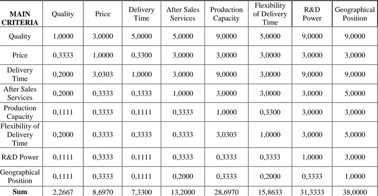
considered for efficiency of suppliers in service industry and appropriate supplier selection have to be choosing to improve the performance of supplier’s since

Mehmed’le yakınlık kurarak ülkede semâ, zikir ve devranı yasaklattığı 1077 (1666) yılından sonra da faaliyetlerini sürdüren Niyâzî-i Mısrî, vaazlarında bu yasağa sebep

In the second stage, the data were replicated with the accumulated data by using artificial immune system clonal selection algorithm and the data were classified by k-means

Çalışma kapsamında oluşturulan araştırma modelinin bağımsız değişkenleri (üst yönetimin desteği, iletişim, tedarikçilerin katılımı, müşterilerin

Sigara kullanımı düşük gelirli sosyoekonomik gruplar arasında yüksek derecede yaygın ve dezavantajlı kullanıcılar da sigaranın zararlarına maruz

SOX yetersizliği oluşturulup daha sonra L-karnitin verilmiş deney grubuna ait sıçan testis dokularının enine kesitinde sadece SOX yetersizliği oluşturulmuş deney grubunun aksine

手術治療及雷射治療,主要乃在眼球之虹膜或小樑組織處切開成為排流管 道。雖然可能發生一些併發症(如白內障或感染),但機會極微。

The fourth chapter is dedicated to the assessment of different modes of resistance pur- sued by the Palestinian outside of the State of Israel as they sought to come to term with