GRADING OF COLON CANCER
a thesis
submitted to the department of computer engineering
and the institute of engineering and science
of bilkent university
in partial fulfillment of the requirements
for the degree of
master of science
By
S¨uleyman Tuncer Erdo˘gan
July, 2009
Assist. Prof. Dr. C¸ i˘gdem G¨und¨uz Demir (Advisor)
I certify that I have read this thesis and that in my opinion it is fully adequate, in scope and in quality, as a thesis for the degree of Master of Science.
Assist. Prof. Dr. Selim Aksoy
I certify that I have read this thesis and that in my opinion it is fully adequate, in scope and in quality, as a thesis for the degree of Master of Science.
Assist. Prof. Dr. Pınar S¸enkul
Approved for the Institute of Engineering and Science:
Prof. Dr. Mehmet B. Baray Director of the Institute
DIAGNOSIS AND GRADING OF COLON CANCER
S¨uleyman Tuncer Erdo˘gan M.S. in Computer Engineering
Supervisor: Assist. Prof. Dr. C¸ i˘gdem G¨und¨uz Demir July, 2009
In our century, the increasing rate of cancer incidents makes it inevitable to em-ploy computerized tools that aim to help pathologists more accurately diagnose and grade cancerous tissues. These mathematical tools offer more stable and objective frameworks, which cause a reduced rate of intra- and inter-observer variability. There has been a large set of studies on the subject of automated cancer diagnosis/grading, especially based on textural and/or structural tissue analysis. Although the previous structural approaches show promising results for different types of tissues, they are still unable to make use of the potential infor-mation that is provided by tissue components rather than cell nuclei. However, this additional information is one of the major information sources for the tissue types with differentiated components including luminal regions being useful to describe glands in a colon tissue.
This thesis introduces a novel structural approach, a new type of constrained Delaunay triangulation, for the utilization of non-nuclei tissue components. This structural approach first defines two sets of nodes on cell nuclei and luminal regions. It then constructs a constrained Delaunay triangulation on the nucleus nodes with the lumen nodes forming its constraints. Finally, it classifies the tissue samples using the features extracted from this newly introduced constrained Delaunay triangulation.
Working with 213 colon tissues taken from 58 patients, our experiments demonstrate that the constrained Delaunay triangulation approach leads to higher accuracies of 87.83 percent and 85.71 percent for the training and test sets, respectively. The experiments also show that the introduction of this new structural representation, which allows definition of new features, provides a more robust graph-based methodology for the examination of cancerous tissues and
better performance than its predecessors.
Keywords: Constrained Delaunay triangulation, histopathological image analysis, automated cancer diagnosis and grading, colon cancer, adenocarcinoma.
KOLON KANSER˙IN˙IN KISITLI DELAUNAY
¨
UC
¸ GENLEMES˙I ˙ILE TES¸H˙IS˙I VE
SINIFLANDIRILMASI
S¨uleyman Tuncer Erdo˘gan Bilgisayar M¨uhendisli˘gi, Y¨uksek Lisans Tez Y¨oneticisi: Y. Do¸c. Dr. C¸ i˘gdem G¨und¨uz Demir
Temmuz, 2009
Y¨uzyılımızda artan kanser vakaları, bilgisayar destekli ara¸cların kullanımını ka¸cınılmaz kılmı¸stır; bunlar patologların kanserli dokulara daha kesin tanı koy-malarına ve sınıflandırkoy-malarına yardımcı olmayı ama¸clamaktadır. Bu matema-tiksel ara¸clar, daha tutarlı ve nesnel yapılar sunarak g¨ozlemci-i¸ci ve g¨ozlemciler-arası de˘gi¸skenli˘gi azaltmaya olanak sa˘glar. G¨un¨um¨uzde, ¨ozellikle dokusal ve/veya yapısal doku analizi temelli otomatik kanser tanı ve sınıflandırması ¨uzerine ¸cok miktarda ¸calı¸sma bulunmaktadır. ¨Onceki yapısal yakla¸sımların farklı tipte dokular i¸cin umut verici sonu¸clar g¨ostermelerine ra˘gmen, bu yakla¸sımlar h¨ucre ¸cekirde˘gi dı¸sındaki doku bile¸senlerinden sa˘glanabilecek potansiyel bilgiyi kullana-bilmekten yoksundurlar. Hˆalbuki bu ek bilgi, farklıla¸smı¸s bile¸senlerden olu¸san doku tipleri i¸cin ana bilgi kaynaklarından birisini olu¸sturmaktadır; ¨orne˘gin l¨umen b¨olgeleri, kolon dokusu i¸cindeki bezleri tanımlamaya yardımcı olmaktadır.
Bu tez ¸calı¸sması, h¨ucre ¸cekirde˘gi dı¸sındaki doku bile¸senlerinin kullanımı i¸cin yeni bir yapısal yakla¸sımı, yeni bir ¸ce¸sit kısıtlı Delaunay ¨u¸cgenlemesini, ortaya koymaktadır. Bu yapısal yakla¸sım ¨oncelikle h¨ucre ¸cekirdekleri ve l¨umen b¨olgeleri ¨uzerinde iki d¨u˘g¨um k¨umesi tanımlar. Daha sonra, l¨umen d¨u˘g¨umleri kısıtları olu¸sturacak ¸sekilde, ¸cekirdek d¨u˘g¨umleri ¨uzerinde bir kısıtlı Delaunay ¨u¸cgenlemesi olu¸sturur. Son olarak, bu yeni tanımlanan kısıtlı Delaunay ¨u¸cgenlemesinden ¸cıkarılacak ¨oznitelikleri kullanarak doku ¨orneklerini sınıflandırır.
Elli sekiz farklı hastadan alınan 213 kolon doku ¨orne˘gi ¨uzerinde ger¸cekle¸stirdi˘gimiz deneyler, kısıtlı Delaunay ¨u¸cgenlemesi yakla¸sımı ile e˘gitim k¨umesi i¸cin y¨uzde 87.83, test k¨umesi i¸cinse y¨uzde 85.71 gibi y¨uksek do˘gruluk de˘gerleri elde edildi˘gini ortaya koymu¸stur. Ayrıca deneylerimiz, yeni ¨ozniteliklerin
tanımlanmasına izin veren bu yeni yapısal g¨osterimin, kanserli dokuların incelen-mesi i¸cin daha g¨urb¨uz bir ¸cizge-tabanlı y¨ontem oldu˘gunu ve ¨onceki y¨ontemlere g¨ore daha y¨uksek ba¸sarı sa˘gladı˘gını g¨ostermektedir.
Anahtar s¨ozc¨ukler : Kısıtlı Delaunay ¨u¸cgenlemesi, histopatolojik g¨or¨unt¨u analizi, otomatik kanser te¸shisi ve sınıflandırılması, kolon kanseri, adenokarsinom.
“Clouds are not spheres, mountains are not cones, coastlines are not circles, and bark is not smooth, nor does lightning travel in a straight line.” (Mandelbrot, 1983).
The subject of science is too broad for one person to be expert in all of its aspects. I thank my master, Assist. Prof. Dr. C¸ i˘gdem G¨und¨uz Demir for her special competence in computer sciences and constant support of me throughout this process, and Prof. Dr. Cenk S¨okmens¨uer for his consultancy on medical knowledge. I would also thank all of the members of my thesis committee; Assist. Prof. Dr. Selim Aksoy and Assist. Prof. Dr. Pınar S¸enkul for kindly agreeing to be in my thesis committee. I also thank T ¨UB˙ITAK-B˙IDEB and the project under the number T ¨UB˙ITAK 106E118 for their financial support to me and our project.
I am extremely grateful to my closest friends for their guidance, encourage-ment, and just standing by me: ˙Imran Ak¸ca, Akın Avcı, Ay¸ca Ak¸cay, Bahadır Bebek, Ceren Bebek, Leyla Bilge, Murat Bo˘gazkesenli, O˘guzhan C¸ elebi, Pınar Do˘gan, Hayrettin G¨urk¨ok, Burcu Kafa, Bahadır Kemalo˘glu, Barı¸s Korkut, Alp Manyas, C¸ a˘gla Okur, Erkan Okuyan, Ya˘gmur ¨Okten, Melih ¨Ozbeko˘glu, Cihan
¨
Ozt¨urk, Mustafa Pelit, Akif Burak Tosun, ¨Omer Sezgin U˘gurlu, Hilal Zitouni, and the rest of my friends, who are the most beautiful people in the world.
This thesis, which you are holding in your hands right now, is created on a tough, thorny, everlasting path. The publication of this thesis would be im-possible without the endless generosity, patience, care, and love of my parents, Nebahat and Mehmet Erdo˘gan, my sister T¨ulay Erdo˘gan, and my future wife, Beng¨u Okur. I am deeply indebted to them for just being who they are.
S. Tuncer Erdo˘gan July 2009
1 Introduction 1
1.1 Motivation . . . 4
1.2 Contribution . . . 6
1.3 Organization of the Thesis . . . 8
2 Background 10 2.1 Medical Terminology . . . 10
2.1.1 Colon tissues . . . 10
2.1.2 Colon adenocarcinoma . . . 12
2.2 Previous Studies on Tissue Analysis . . . 13
2.2.1 Textural features . . . 13
2.2.2 Structural features . . . 16
2.3 Constrained Delaunay Triangulations . . . 23
3 Methodology 28 3.1 Node Segmentation . . . 29
3.1.1 Transforming into Lab color space . . . 31 3.1.2 K-means clustering . . . 31 3.1.3 Preprocessing . . . 32 3.1.4 Circle-fit transform . . . 34 3.2 Graph Generation . . . 35 3.2.1 Delaunay triangulation . . . 37
3.2.2 Constrained Delaunay triangulation . . . 39
3.3 Feature Extraction . . . 41
3.3.1 Connectivity based features . . . 43
3.3.2 Component related features . . . 46
3.3.3 Spatial features . . . 47
3.4 Classification and Feature Reduction . . . 47
3.4.1 Classification . . . 48 3.4.2 Feature reduction . . . 51 4 Experimental Results 54 4.1 Experimental Setup . . . 54 4.2 Results . . . 55 4.2.1 Parameter selection . . . 55
4.2.2 Feature selection and reduction . . . 61
4.3 Discussion . . . 84
4.3.1 Parameter selection . . . 84
4.3.2 Feature definition and selection . . . 85
4.3.3 Complexity of algorithms . . . 88
5 Conclusion and Future Work 89
Bibliography 92
1.1 Histopathological images of colon tissues . . . 5
1.2 The boundaries of individual cell nuclei of colon tissues . . . 7
1.3 A sample Delaunay triangulation built onto nuclei structures of colon tissues . . . 9
2.1 The layout of a colon tissue stained with the H&E technique . . . 11
2.2 A Voronoi diagram of random points . . . 17
2.3 Delaunay triangulation . . . 18
2.4 Delaunay triangulation together with its corresponding Voronoi diagram . . . 19
2.5 Various structural types of computational geometry . . . 22
2.6 Delaunay triangulation & Constrained Delaunay triangulation . . 24
3.1 Overall system architecture . . . 29
3.2 Colon tissue samples . . . 30
3.3 Clustered biopsy samples . . . 33
3.4 Circle-fit transform . . . 36 xii
3.5 Delaunay triangulation constructed on only the purple nodes . . . 38 3.6 Delaunay triangulation constructed on both the white and purple
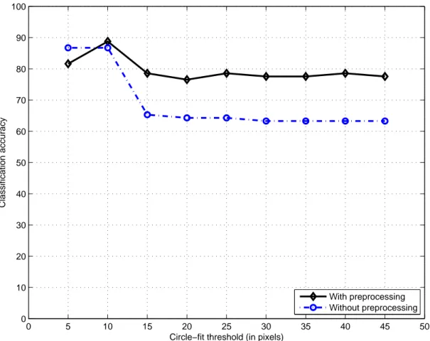
nodes . . . 40 3.7 Constrained Delaunay triangulation . . . 42 3.8 An isolated node in a luminal area . . . 44 3.9 The hyperplane separating two data sets in 2-dimensional space. . 49 3.10 Separable classification with kernel mapping. . . 50 4.1 Classification results with and without preprocessing . . . 57 4.2 Circle representations of the tissue image shown in Figure 3.2a . . 58 4.3 Classification results for the test set with varying values of SVM
cost parameter C between 1 and 10000. These results are obtained with preprocessed data. . . 60 4.4 Classification results for the test set with varying values of SVM
cost parameter C between 1 and 2000. These results are obtained with preprocessed data. . . 61 4.5 Classification results in PCA for the training set. These results are
obtained by choosing the SVM cost parameter C individually with 10-fold cross-validation in each iteration and with preprocessed images. . . 65 4.6 Classification results in PCA for the test set. These results are
obtained by choosing the SVM cost parameter C individually with 10-fold cross-validation in each iteration and with preprocessed images. . . 66 4.7 Classification results in forward selection . . . 69
4.8 Classification results in backward elimination . . . 73 4.9 Test accuracies of constrained Delaunay triangulation and
Delau-nay triangulation. These results are obtained by choosing the SVM cost parameter C individually with 10-fold cross-validation in each iteration and with preprocessed images. . . 76 4.10 The difference in test accuracies of constrained Delaunay
triangu-lation and Delaunay triangutriangu-lation. (See Figure 4.9) . . . 77 4.11 The test set accuracies obtained by constrained Delaunay
triangu-lation and Delaunay triangutriangu-lation in healthy tissues. (See Figure 4.9) . . . 78 4.12 The test set accuracies obtained by constrained Delaunay
triangu-lation and Delaunay triangutriangu-lation on low-grade cancerous tissues. (See Figure 4.9) . . . 79 4.13 The test set accuracies obtained by constrained Delaunay
triangu-lation and Delaunay triangutriangu-lation on high-grade cancerous tissues. (See Figure 4.9) . . . 80 4.14 Test accuracies of constrained Delaunay triangulation and
Delau-nay triangulation. These results are obtained by choosing the SVM cost parameter C individually with 10-fold cross-validation and us-ing non-preprocessed images. . . 82 4.15 The difference between in test accuracies of constrained Delaunay
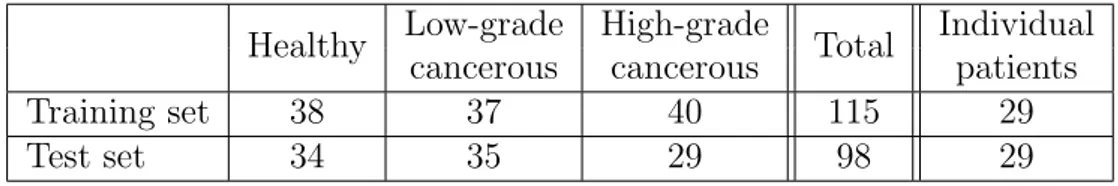
1.1 Leading causes of death worldwide . . . 2 3.1 The list of extracted features . . . 48 4.1 Number of samples in the training and test sets . . . 55 4.2 The confusion matrix and the training set classification accuracy of
the constrained Delaunay triangulation approach with the circle-fit threshold value being selected as 10. These results are obtained with using preprocessed images. . . 63 4.3 The confusion matrix and the test set classification accuracy of
the constrained Delaunay triangulation approach with the circle-fit threshold value being selected as 10. These results are obtained with using preprocessed images. . . 63 4.4 The confusion matrix and the training set classification accuracy of
the Delaunay triangulation approach with the circle-fit threshold value being selected as 10. These results are obtained with using preprocessed images. . . 64 4.5 The confusion matrix and the test set classification accuracy of
the Delaunay triangulation approach with the circle-fit threshold value being selected as 10. These results are obtained with using preprocessed images. . . 64
4.6 Forward selection results for 10-fold cross-validation . . . 67 4.7 Forward selection results for the training set . . . 68 4.8 Forward selection results for the test set . . . 68 4.9 Selected features and the corresponding test set accuracies in
for-ward selection. Our manually selected features are written in italics. 70 4.10 Backward elimination results for 10-fold cross-validation . . . 71 4.11 Backward elimination results for the training set . . . 71 4.12 Backward elimination results for the test set . . . 72 4.13 Eliminated features and the corresponding test set accuracies in
backward elimination. . . 72 4.14 Training set accuracy obtained by the constrained Delaunay
trian-gulation. The circle-fit threshold value is selected as 10. . . 74 4.15 Test set accuracy obtained by the constrained Delaunay
triangu-lation. The circle-fit threshold value is selected as 10. . . 74 4.16 Training set accuracy obtained by the Delaunay triangulation. The
circle-fit threshold value is also selected as 10. . . 75 4.17 Test set accuracy obtained by the Delaunay triangulation. The
circle-fit threshold value is also selected as 10. . . 75 4.18 The list of features . . . 86 4.19 Training set accuracy obtained by the constrained Delaunay
trian-gulation. . . 87 4.20 Test set accuracy obtained by the constrained Delaunay
triangu-lation. . . 87 4.21 Training set accuracy obtained by the Delaunay triangulation. . . 87
4.22 Test set accuracy obtained by the Delaunay triangulation. . . 87 4.23 Complexity of algorithms . . . 88 5.1 Training set accuracy obtained by the constrained Delaunay
tri-angulation. In this experiment, the common features that are also available to standard Delaunay triangulation are used for the train-ing and classification. . . 90 5.2 Test set accuracy obtained by the constrained Delaunay
triangula-tion. In this experiment, the common features that are also avail-able to standard Delaunay triangulation are used for the training and classification. . . 91 A.1 Implementation details of our approach . . . 108
Introduction
Cancer, which is also known as malignant neoplasm, is a serious, lethal class of human diseases that occurs with the ungoverned expansion, division, and spread of abnormal cells. 12.5 percent of deaths worldwide is due to cancer and cancer results in more deaths than AIDS, tuberculosis, and malaria combined, as pre-sented in Table 1.1. It is also the second leading cause of death in economically developed countries, following heart diseases, and the third leading cause of death in developing countries, right after heart diseases and diarrhoeal diseases [52].
Cancer affects a variety of organs or systems. Most types of cancer, such as prostate, breast, and colorectal, form a tumor and affect the organ they originate from. On the other hand, some types do not form a tumor, like leukemia. One of the most common tumor-forming-cancer type is colon cancer, which is also named as colorectal cancer or large bowel cancer. According to studies, it is the third leading cause of cancer-related deaths in developed countries for both men and women [52].
According to World Health Organization, one third of these cancer incidents could be reduced by enforcing cancer-preventing strategies [127]. Another third could be cured if they are diagnosed early and treated adequately. Regular screen-ing examinations by health care professionals may prevent the cancer to be formed and result in the removal of pre-malignancy growths. Considering the occurrence
Worldwide Developing Developed
Rank % Rank % Rank %
Heart diseases 1 19.6 1 18.1 1 28.6
Malignant neoplasms 2 12.5 3 10.2 2 26.2
CV diseases 3 9.6 4 9.5 3 9.9
Lower resp. infections 4 6.7 5 7 4 4.4
COPD* 5 4.8 8 4.9 5 3.8
HIV/AIDS 6 4.6 6 5.3 - 0.3
Perinatal conditions** 7 4.5 7 5.1 - 0.4
Diarrhoeal diseases 8 3.2 2 16.1 - 0.1
Tuberculosis 9 2.9 9 3.3 - 0.2
Road traffic accidents 10 2.0 - 2.2 9 1.5
Malaria 11 2.1 10 2.5 - 0.0
Diabetes mellitus 12 1.7 - 1.6 7 2.6
Suicide 13 1.6 - 1.5 8 1.6
Cirrhosis of the liver 14 1.4 - 1.4 10 1.5
Measles 15 1.4 - 1.6 - 0.0
The number zero in a cell indicates a non-zero estimate of less than 500 deaths. *COPD is chronic obstructive pulmonary disease.
**This cause category includes “causes arising in the perinatal period” as defined in the International Classification of Diseases, principally low birthweight, prematurity, birth as-phyxia, and birth trauma, and does not include all causes of deaths occurring in the perinatal period.
Source: Lopez AD, Mathers CO, Ezzati M, et al. Global and regional burden of dis-ease and risk factors, 2001: Systematic analysis of population health data. Lancet. 2006;367(9524):1747-57.
Table 1.1: Leading causes of death worldwide (in developing and developed coun-tries), 2001
and death rate of cancer throughout the world, the value of early and accurate detection of the cancerous tissues and the selection of the correct treatment plan are very important.
It should be noted that the correct treatment selection is always the key to recovery and convalescence. One of the main factors that affects the treatment selection is accurate diagnosis and grading of cancer. In the current practice of medicine, several methods have been proposed for cancer diagnosis. The first cat-egory of these methods consists of medical imaging techniques, such as magnetic resonance imaging (MRI), nuclear MRI (NMRI), computed tomography (CAT scan), and positron emission tomography (PET scan). These techniques are used to diagnose the cancerous regions, but they are incapable of providing reliable information for grading process. The second group of formerly proposed can-cer diagnosis methods is molecular diagnosis [33, 38, 65, 78, 110]. This type of diagnostic methods is not for widespread use, due to the fact that genetic infor-mation is highly complicated and there exists a requirement for both specialists and complex and costly apparatus.
For these reasons, in the current practice of medicine, histopathological ex-amination is still the gold standard for both cancer diagnosis and grading. For the examination, a sample tissue, which is called biopsy, is surgically removed from a patient. Afterwards, the biopsy is placed onto a glass slide and stained with a special technique to enhance contrast in the microscopic image. In the histopathological examination, a pathologist examines the structure of the tis-sue to determine whether it is cancerous or not. If it is cancerous, s/he also determines the type and grade of cancer.
Histopathological examination yields valuable clinical information and pro-vides accuracy both in diagnosis and grading [14, 22, 63, 69]. Neverthless, cancer diagnosis is still a major challenge for cancer specialists worldwide [95, 102]. The main drawback of the histopathological examination is that the analysis is sub-jective to visual interpretation and experience of the pathologist, especially in grading process [3, 36, 114].
reliable decisions, computer-aided diagnosis has been proposed. Computer-aided diagnosis is becoming more robust and reliable with the development of novel ap-proaches and evolution of algorithms in the long run. They also gain momentum and become widely accepted with the falling prices and improvement of hardware infrastructure. Cheap processing power is coming into the picture as a natural result of these maturing computer technologies. However, the existing systems present their own challenges and have their own shortcomings.
1.1
Motivation
Ongoing development in computer technologies has already been canalized into cancer research projects. Many studies have been proposed to use computerized image analysis to support pathologists and to reduce the variability between the decisions of the pathologists. In these studies, a tissue is represented with a set of mathematical features and these features are then used in automated diagnosis and grading process. These studies mainly focus on textural and/or structural tissue analysis.
In the first group of these studies, the texture of the entire tissue is character-ized with a set of textural features such as those calculated from co-occurrence ma-trices [40, 43, 103], run-length mama-trices [126], multiwavelet coefficients [67, 126], fractal geometry [7, 37, 44], and optical density [43, 126].
In the second group, the cell distribution within a tissue is represented as a graph and structural features are extracted from this graph representation. Pre-vious studies consider the locations of cell nuclei as nodes to generate such graphs including Delaunay triangulations [40, 72], Gabriel graphs [112, 124], minimum spanning trees [18, 124], and probabilistic graphs [32].
The major drawback of the previous graph-based studies is their incapability of using potential information that is provided by other tissue components rather than cell nuclei. Because of their nature, such information becomes useful espe-cially for the representation of the tissue types where tissues consist of hiearchical
Lumen
Epithelial cell
(a) Healthy (b) Healthy
(c) Low-grade cancerous (d) Low-grade cancerous
(e) High-grade cancerous (f) High-grade cancerous
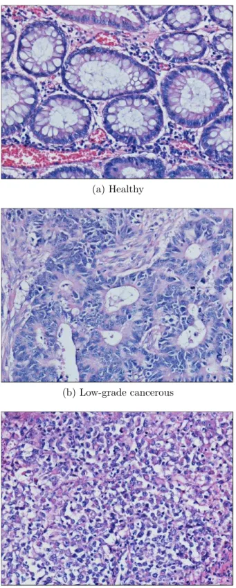
Figure 1.1: Histopathological images of colon tissues. These tissues are stained with the hematoxylin-and-eosin technique, which is routinely used to stain biop-sies in hospitals.
structures. For example, in colon tissues, epithelial cells are lined up around a lumen to form a glandular structure. The gland architecture for a normal colon tissue is shown in Figures 1.1a and 1.1b with the lumen and an epithelial cell of a single gland being indicated with arrows. Colon adenocarcinoma, which accounts for 90–95 percent of all colorectal cancer incidents, distorts the gland formations. At the beginning, the degree of distortion is lower such that the gland forma-tions are well to moderately differentiated; examples of such low-grade cancerous tissues are shown in Figures 1.1c and 1.1d. Then the distortion level becomes higher such that the gland formations are only poorly differentiated; examples of such high-grade cancerous tissues are shown in Figures 1.1e and 1.1f. For the automated diagnosis and grading of colon cancer, these distortions should be quantified. Obviously, for a colon tissue, the additional information obtained from luminal components facilitates better tissue quantification compared to the case where the information is obtained from only cellular/nuclear tissue components. Another drawback of the previous graph-based techniques is their require-ment of high-quality segrequire-mentation. Accurate extraction of nuclei information is crucial for the proposed algorithms and it surely ensures higher and more reli-able recognition rates, because the algorithms make use of spatial information provided by these nodes. However, in the image magnification on which a graph is extracted, the boundaries of individual cell nuclei of colon tissues are occasion-ally uncertain and they are even inseparable by an expert. Figure 1.2 points out the indistinguishability of some nuclei groups. Therefore, An alternative node definition algorithm is necessary to eliminate the requirement of a high-quality segmentation.
1.2
Contribution
The formation of glandular structures is characterized with the locations of cells and luminal regions with respect to each other and it affects the decisions of pathologists for diagnosis and grading. Thus, it should also affect the results acquired by computer-aided diagnosis systems. However, traditional graph-based
Figure 1.2: In the image magnification on which a graph is extracted, the bound-aries of individual cell nuclei of colon tissues are occasionally uncertain.
approaches ignore this fact and use the information provided by the features that are extracted from any type of graph which is just built onto cell nuclei structures. On the contrary, for better characterization of a tissue, it is beneficial to define representative graph nodes on luminal regions rather than defining them only on nuclear regions. These nodes can be used in such a way that they facilitate the luminal information for recognition systems.
In this thesis, we report a new structural method that considers the loca-tions of both nuclear and luminal components for tissue representation. Unlike the previous studies that use the standard Delaunay triangulation and its corre-sponding Voronoi diagram on nuclei, we propose to use a new type of constrained Delaunay triangulation (and its corresponding Voronoi diagram) to represent the tissue. In this representation, we assign edges between nuclear components where luminal components form the constraints. Then we define a new set of structural features on this constrained Delaunay triangulation, and use these features in the classification of colon tissues. The constrained Delaunay triangulation of an exemplary colon tissue image, which is shown in Figure 1.3e, and its correspond-ing Voronoi diagram are shown in Figures 1.3a and 1.3b, respectively. In their construction, both nuclear and luminal components are considered as opposed to the construction of standard Delaunay triangulation and Voronoi diagram where only nuclei components are utilized but non-nuclei components are not consid-ered. For the same tissue image, the standard Delaunay triangulation and its
corresponding Voronoi diagram are shown in Figures 1.3c and 1.3d, respectively. In this representation, a set of circular primitives, formed by a technique called circle-fit transform [115], is used as the nodes of the triangulation. With the help of this approach, the problem that arises from the necessity of using classical and inefficient segmentation algorithms is alleviated. Furthermore, images with lower resolution are sufficient for the proposed circle-fit transform, which decreases the CPU-time.
1.3
Organization of the Thesis
The remaining of this thesis is organized as follows: In the first section of the following chapter, a brief explanation of medical background and terminology is presented. The following section exposes the previous studies in this research area of cancer diagnosis, emphasizing their disadvantages for colon tissues, and revises the related work on the use of constrained Delaunay triangulation. Chapter 3 explains the details of our proposed structural method. Consequently, Chapter 4 describes the experimental framework and analyzes the experimental results. Finally, Chapter 5 provides a summary of our work and discusses the future directions of our study.
(a) Constrained Delaunay triangulation (b) Voronoi diagram of constrained Delau-nay triangulation
(c) Delaunay triangulation (d) Voronoi diagram of Delaunay triangu-lation
(e) Tissue image
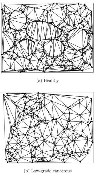
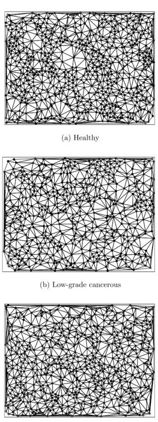
Figure 1.3: A sample Delaunay triangulation built onto nuclei structures of colon tissues. It can be observed that nuclei around or in the middle of a luminal region are connected to each other in the traditional Delaunay triangulation, where they are not suppossed to be.
Background
In this chapter, the underlying medical terminology of this thesis is presented. The structure of colon tissues, staining process, structural changes in different grades of colon cancer are some of the topics investigated in the first section.
Following the medical background, a brief overview of the previous computa-tional methods for the diagnosis of cancerous tissues other than the graph-based methods is given. Afterwards, broader knowledge on the subject of graph-based methods is presented. Finally, other applications of constrained Delaunay trian-gulation are overviewed.
2.1
Medical Terminology
2.1.1
Colon tissues
The colon, or the large intestine or large bowel, is the last portion of the digestive track and is responsible for extracting water and electrolytes from feces just before they are excreted. The remaining solid waste is also stored until leaving the body through the anus.
When cancer is suspected, a variety of methods can be applied to detect the status of a tissue. In the current practice of medicine, histopathological examina-tion is the gold standard. For diagnostic evaluaexamina-tion, a sample tissue is surgically removed from the patient. This procedure is called a biopsy. The biopsy specimen is sent to a pathologist for the microscopic examination.
In the next step, sections are taken from the biopsy specimen and they are stained with special chemical compounds for the ease of visibility at mi-croscopic level. In this thesis, we use the images of colon tissues stained with the hematoxylin-and-eosin technique (H&E). This staining technique is a conven-tional one and is routinely used to stain tissues at hospitals. In this technique, hematoxylin is the active ingredient of the staining solution and colors nucleic acids with a blue-purple hue. On the other hand, alcohol-based acidic eosin col-ors eosinophilic structures (i.e., proteins) with bright pink. Consequent view un-der the microscope carries the characteristic blue-stained nuclei and pink-stained stroma [47, 75]. Therefore the color spectra of the images of tissues stained with the H&E technique are commonly rich of blue-purple, pink, and white pixels.
Gland borders
Arbitrary empty region Lamina propria
Epithelial cell nucleus
Luminal area Epithelial cell cytoplasm
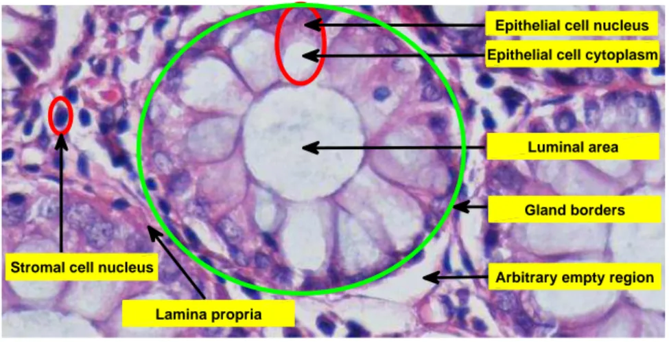
Stromal cell nucleus
Figure 2.1: The layout of a colon tissue stained with the H&E technique Figure 2.1 exhibits the layout of a colon tissue stained with the H&E tech-nique. Cells in a tissue could be grouped into two: epithelial cells and stromal cells. Simple columnar, non-ciliated epithelial cells form the epithelium tissue of
colon [96]. A sample epithelial cell is highlighted in Figure 2.1 with a red circle, of which the dark purple region constitutes its nucleus, and the lighter white section next to nucleus is cytoplasm. A group of epithelial cells is lined up around an oval vacant region called luminal area to form a gland all together. Luminal area of a gland body is also marked in this figure. Also, there may exist an arbitrary vacant region around or inbetween gland bodies, which is just an artifact that arises from the sectioning procedure.
The remaining region outside the gland bodies consists of loose connective tissue, which makes up the support structure of biological tissues and holds all of the structures in the tissue together. The cells found in the loose connective tissue could be called as stromal cells. These are diffused around glandular bodies and they are not part of a gland structure. Moreover, the pink area around stromal cells is composed of noncellular material called lamina propria.
2.1.2
Colon adenocarcinoma
Colon tissues may easily become cancerous in course of time, due to the fact that an uninterrupted stress provided by storaged solid waste is present. The risk fac-tors of colon cancer also include a diet low in fiber and high in fat, certain types of colorectal polyps, inflammatory bowel disease such as Crohn’s disease or ulcera-tive colitis, smoking, alcohol, and some inherited genetic disorders transmitted at birth. Improper nutrition habits tending to pervade in developing countries, as a natural result of intense life routines, heighten the risk of colon cancer. Colon ade-nocarcinoma is its most common type, which accounts for approximately 90 − 95 percent of all colon cancers.
In a typical healthy colon tissue, there exists an harmonious and coherent composition of gland bodies and loose connective tissue. With the abnormal growth and division of cells, due to the aforementioned reasons, tumors may grow out of healthy tissues and consistent structure of colon may get corrupted. A tumor can be benign (non-cancerous) or malignant (cancerous). If the tumor is malignant and has expansionary properties, it may diffuse into other organs and
become lethal in case of not being cured. Tumor grading is the scheme used to catalogue the status of cancer cells in the sense of how anomalistic they appear and how rapidly the tumor is likely to grow and spread.
Tumors may be graded on four-tier, three-tier and two-tier scales [46]. In two-tier grading scheme, which is the scheme used in this thesis, there are
• Low-grade cancer, in which the glands are well to moderately differentiated, and
• High-grade cancer, in which the glands are only poorly differentiated.
2.2
Previous Studies on Tissue Analysis
Many studies have been proposed to use computerized image analysis to support the pathologists and to reduce the variability between the decisions of pathol-ogists. Previous studies have focused on different aspects of image process-ing. Mainly, these studies made use of textural and structural representation of histopathological images. Less number of studies used other types of informa-tion such as color based features and/or morphological features. In this chapter, we will overview the fundamental textural and structural features of histopatho-logical image processing.
2.2.1
Textural features
In the first group of previous studies, the texture of the entire tissue is charac-terized with a set of textural features such as those calculated by the following approaches:
Co-occurrence matrix : Co-occurrence matrix is accumulation of pixel level data which is the distribution of co-occurring values at varying offsets. It is initially defined by Haralick et al. in 1973 [61]. The other known identities are
co-occurrence distribution, gray-level co-occurrence matrix (GLCM), and spatial dependence matrix. For a w × h image I parameterized by an offset (∆x, ∆y), the co-occurrence matrix C is defined in Equation 2.1:
C (i, j) = w X p=1 h X q=1 1, if I (p, q) = i and I (p + ∆x, q + ∆y) = j 0, otherwise (2.1)
Co-occurrence matrix is sensitive to rotation, so the use of a set of offsets corresponding to 0, 45, 90 and 135 degrees results in a degree of rotational invari-ance. Also, the value of the image is generally referred to the gray-scale value of the specified pixel. However, in literature, co-occurrence matrices have been commonly used to extract texture information not only from gray-scale images [8, 18, 42, 43, 60, 103, 124, 126], but also from colored images [107, 108].
The resulting co-occurrence matrices are not sufficient to be analyzed by them-selves, so many features are extracted from these matrices such as inertia, en-tropy, total energy, angular second moment, contrast, correlation, variance, sum average-variance-entropy, and difference variance-entropy-moment, also known as Haralick’s features [61].
Run-length matrix : Gray-level run-length method has been initially defined by Galloway [51] and its features are then extended by Chu et al. [19]. It is another effective way of accessing higher order statistical texture features [2]. Although it is shown that run-length method is slightly less adequate for texture analysis comparing to other methods [21, 122], later improvements consolidate the employability of the algorithm [113].
Galloway’s proposition of run-length matrix is as follows: For a given image, a run-length matrix p (i, j) is defined as the number of runs with pixels of gray-level i and run length j, where a run is defined as a set of linearly sequential pixels belonging to the same intensity. In literature, there exist some features defined on run-length matrices such as short runs emphasis, long runs emphasis, gray-level non-uniformity, run length non-uniformity, run percentage, low gray-level run
emphasis, and high gray level run emphasis [113]. Later, additional features like short run low gray-level emphasis, short run high gray-level emphasis, long run low gray-level emphasis, and long run high gray-level emphasis are also defined on these matrices [26]. High gray-level run emphasis (HGRE) feature is presented as an example in Equation 2.2: HGRE = 1 nr M X i=1 N X j=1 p (i, j) · i2 (2.2)
These features are also used for the diagnosis and grading of cancerous tis-sues in previous studies conducted by Weyn et al. [125] and Bibbo et al. [8]. Extracted features are used for classification with KNN classification [126], his-togram method [125], or three-way discriminant analysis [8].
Multiwavelet coefficients : Wavelets are special classes of functions that are used to represent data or other functions by dividing them into different scale components [54]. They have very important applications especially in image (data) compression and denoising (image enhancement) [5, 15, 24, 25, 27, 55, 66, 83, 87, 90, 93, 99]. The details of the wavelets are out of the scope of this thesis and references will be left to the reader for future investigation.
Three classes in which wavelet transforms are divided are continuous, discrete, and multiresolution-based wavelets. Multiwavelets are superior to former classes and possess additional properties like orthogonality, symmetry, and vanishing moments, which are known to be important in signal and image processing, and resulting in being advantageous over scalar ones [1, 111, 116].
Multiwavelet coefficients enable researchers to lower the dimension of data and analyze it through some features. Some set of features like energy and entropy can be extracted from multiwavelet coefficients and they are also used to improve accuracy on colon image classification in previous studies [29, 67, 123, 126].
Fractal dimension : Mandelbrot defined a fractal as an image and/or geo-metric shape that appears identical and repeats itself as it is scaled down, which
cannot be represented by classical geometry [80]. In fractal geometry, the fractal dimension, D, is a measure of complexity which gives an indication of how a fractal appears to fill space as it is zoomed further. The statistical quantity D is acquired with the following equation, where N (²) is the number of self-similar structures of diameter ² necessary to cover the structure:
D = lim ²→0 log N (²) log 1 ² (2.3) Previous studies on histopathological image analysis make use of fractal di-mension information to improve accuracy achieved by other methods [7, 37, 44]. Although the analysis shows that fractal dimension is highly correlated with fea-tures like correlation and entropy, it is shown that fractal dimension information improves sensitivity and can be useful for automated techniques in clinical prac-tice in the future [44].
2.2.2
Structural features
In the second group of previous studies, the cell distribution within a tissue is represented as a graph or diagram and structural features are extracted from these representations. These studies are mainly focused on the following repre-sentations:
Voronoi diagram : Voronoi diagram is defined as the decomposition of a regular plane with n data points into convex polygons such that each polygon encloses its unique origin point and every point inside is closer to the origin point of its polygon than any other data points. For each point pi in the set of coplanar
points P , a boundary enclosing all the intermediate points lying closer to the corresponding origin point pi than other points in the set P can be drawn. Each
one of the enclosing points are called Voronoi polygons. Figure 2.2 demonstrates the schema of a Voronoi diagram constructed on 50 random points.
Figure 2.2: A Voronoi diagram of random points. It is observable that every single point has its own mutually disjoint convex polygon, i.e., Voronoi polygon. was trying express the division of universe by stars in 1644 [88]. The original definition of Voronoi diagrams goes back to 1850 with Lejeune Dirichlet [35], but later, Voronoi extended the investigation of Voronoi diagrams to higher dimen-sions in 1907 [120]. Due to its history, Voronoi diagrams are also called Dirichlet tessellation (also medial axis transform, Wigner-Seitz zones, domains of action, and Thiessen polygons [98]). Each mutually disjoint convex polygon of a Voronoi diagram is called Dirichlet regions, Thiessen polytopes, or Voronoi polygons.
Voronoi diagram has become a classical approach and has been applied across many studies in computer vision and image analysis [6, 45, 88, 98]. Intrinsically, cancer studies have taken advantage of the Voronoi diagrams [9, 72, 81, 101, 124, 126]. In these studies, the very fundamental features such as area and shape of the polygons are sufficed to ensure the satisfying discriminative power among other types.
Delaunay triangulation : Delaunay triangulation is a special type of graph of which edges satisfies the following rule: The circumcircle of each individual triangle is an empty circle, pointing out that there must not exist any other point inside the circle. The triangulation is named after Boris Delaunay, who defined
it in 1934 [30]. The original formal definition of a single Delaunay triangle for two-dimensional space is as follows:
Definition 1 Let P be a finite set of points. Non-collinear points pi, pj and pk of set P form a Delaunay triangle t if and only if there exists a location x which is equally close to pi, pj and pk and closer to pi, pj, pk than any other pm ∈ P. The location x is the center of a circle which passes through the points pi, pj, pk and contains no other points pm of P. For the 2D space, there exist only one circle which is the circumcircle of t [48].
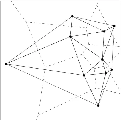
Figure 2.3a visualizes the circumcircle of a single Delaunay triangle. Delaunay triangulation is the dual of Voronoi diagram in R2. It maximizes the minimum interior angle of all of the angles of the triangles in the triangulation. Delaunay triangulation of ten random points is visualized in Figure 2.3b, and presented together with its corresponding Voronoi diagram in Figure 2.4:
(a) Circumcircle of a Delaunay triangle (b) Delaunay triangulation of ten random points
Figure 2.3: Delaunay triangulation
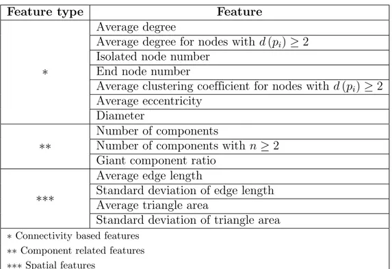
There are many features available to be calculated using Delaunay triangula-tion, since it is a variation of graphs. Most of the features below are also common to the following graph representations, which are to be explained in this section. For each feature type, some statistics such as mean, standard deviation, skewness,
and kurtosis can be calculated over the corresponding feature values, creating a broad selection pool of subfeature types.
Figure 2.4: Delaunay triangulation together with its corresponding Voronoi di-agram. In this figure, dashed lines represent the boundary lines for Voronoi polygons, and the solid lines belong to Delaunay triangulation.
• Length of edges - Features can be defined on the information of distance between the nodes which share a common edge. The feature can be defined on global scale (e.g., the mean of edge lengths), or defined per node (e.g., the standard deviation of edge lengths for each node). An alternative feature can be the distance to nearest neighbors per node (which is connected by an edge) or the distance to the farthermost neighbor [72, 124]. Another modification of the feature can be the average distance to, for instance, the five closest neighbors [71].
• Number of edges - Similar to the previous feature, total number of edges in the entire image or a variation of statistical data per node can be used for classification [72, 124].
• Triangle area - The mean of the triangle area for the entire image or the kurtosis of areas of triangles that share a common vertex per node are two examples of how this feature can be utilized [72].
• Number of triangles - The number of triangles per unit area or per node can be other types of features [72].
• Polarity of the edges - Angles inbetween the edges can also be utilized for polarity information [18].
Not only Delaunay triangulation, but all of the graph types used in the pre-vious studies are built on a set of nodes which, in fact, represents the positional information of nuclei of the tissues. Previous studies have adopted this approach as a general rule and defined features on these graphs [10, 18, 40, 72, 124]. As mentioned before, most of the aforementioned features are also common to these graphs.
Gabriel graphs : Gabriel graph is another type of neighborhood graph which attempts to represent the overall spatial arrangement of the points in a set of P , named after Gabriel who proposed the use of newborn graph in 1969 [50]. It is a subgraph of Delaunay triangulation [94]. Gabriel graph forbids inclusion of any other point to the circle accepting an edge between two points as diameter, unlike the Delaunay triangulation, which defines the circle on three points forming a Delaunay triangle. A Gabriel graph edge is defined as follows:
Definition 2 Let P be a finite set of points. Two points pi and pj of set P are connected by an edge of the Gabriel graph, and they are said to be Gabriel neighbors, if and only if the circle having line segment pipj as its diameter does not contain any other points of P in its interior. DG (P) contains the Gabriel graph of P, GG (P).
A sample Gabriel graph of the point set presented in Figure 2.5a, is given in Figure 2.5c. It is obvious that this Gabriel graph is a subgraph of Delaunay triangulation presented in Figure 2.5b.
Gabriel graphs have been used in various applications, but have not been employed widely in cancer diagnosis applications. Sudbo et al. [112] and Weyn et al. [124] made use of Gabriel graphs to increase accuracy in their work.
Minimum spanning tree : A spanning tree T of connected, undirected, and unweighted graph G is a subgraph that reaches out to all the nodes with n − 1 edges and is a tree, which is a connected graph without cycles. On the other hand, a minimum spanning tree of a weighted graph is the one of the alternative spanning trees with the least total weight. A minimum spanning tree for the given point set is also constructed and presented in Figure 2.5d.
Similar to the Gabriel graphs, the minimum spanning tree are used to improve discriminative power of image analysis systems in the previous studies of Choi et al. [18] and Weyn et al. [124].
Probabilistic graphs : Unlike the previous graph types, probabilistic graphs are constructed by probabilisticly assigning edges between every pair of nodes. Then the cell distribution in a tissue is quantized by the features extracted from these probabilistic graphs [32, 59]. For example, in [32], the probability of the existence of an edge P (u, v) is defined as:
P (u, v) = d (u, v)−α (2.4)
where d (u, v) is the Euclidean distance from node u to node v, and 0 < α ≤ 1 is the parameter that controls the edge density of the graph. Larger values of α increase the number of edges in the graph. Formal definition of these probabilistic graphs is as follows; a sample of a probabilistic graph is given in Figure 2.5f. Definition 3 Let G = (V, E) be a generated graph with V being the set of nodes and E representing the edges of the graph. The binary relation E of V is defined as E = ©(u, v) : r < d (u, v)−α, ∀u, v ∈ Vª, where r is a generated random real number between 0 and 1.
(a) Point set (b) Delaunay triangulation
(c) Gabriel graph (d) Minimum spanning tree
(e) Voronoi diagram with Delaunay triangulation
(f) Probabilistic graph with r = 0.1
weighted, complete graphs without self loops. With the use of augmented graphs in a study by Demir et al. [31], usage of several control parameters are eliminated due to the fact that augmented graphs are complete graphs. Inclusion of all pos-sible edges between every pair of nodes prevents the loss of any kind of existing spatial information. The study revealed a remarkable and exceptional accuracy achieved in the classification of glioma, which is a type of brain cancer.
2.3
Constrained Delaunay Triangulations
As its definition is given earlier in Section 2.2.2, Delaunay triangulations are one of the most commonly used structural entities in the history of mathematics and computational geometry. There exist an extension to Delaunay triangulation, constrained Delaunay triangulation, which satisfies the following properties:
• The prespecified edges that are obliged to be included in the final graph representation appear in the triangulation.
• The triangulation is as close as possible to the Delaunay triangulation. More formally, constrained Delaunay triangulation is originally defined by Chew in [17] as follows:
Definition 4 Let G be a straight-line planar graph. A triangulation T is a con-strained Delaunay triangulation (CDT) of G if each edge of the G is an edge of T and for each remaining edge e of T , there exists a circle C with the following properties: (1) the endpoints of edge e are on the boundary of C, and (2) if any vertex v of G is in the interior of C then it cannot be “seen” from at least one of the endpoints of e (i.e., if you draw the line segments from v to each endpoint of e then at least one of the line segments crosses an edge of G).
Figure 2.6a demonstrates ten points in 2D space. Suppose that the thick lines are the constraint edges and they must appear in the final triangulation. Figure
2.6b shows the conventional Delaunay triangulation calculated with empty-circle rule, disregarding the constraints. On the other hand, Figure 2.6b points out the structuring of constrained Delaunay triangulation. Note that the prespecified edges are included in the final triangulation, and the graph is kept as close as to Delaunay triangulation.
(a) Data points and the con-straint edges
(b) Delaunay triangulation of data points
(c) Constrained Delaunay triangulation of data points and constraint edges
Figure 2.6: Constrained Delaunay triangulation
Constrained Delaunay triangulation is introduced by Lee et al. [74] and Chew [16] separately, but later the definition has been expanded to higher dimensions by other studies [56, 105, 109]. There have been many studies about the con-struction of Delaunay triangulation from scratch and reconcon-struction of deformed or swelled triangulations. Construction of constrained Delaunay triangulation can be achieved via adaptation of proposed methods. Delaunay construction al-gorithms and current succesful adaptations are categorized under three general groups:
• Divide and conquer algorithms: In divide and conquer algorithms, the in-put set is partitioned into subsets, the smaller subsets of the inin-put set are triangulated individually and the resulting triangulations are merged in the final step. These type of algorithms are generally sophisticated and require complex data types, but they are well suited for parallel program-ming. Chew [16], Dwyer [41], Ruppert [97], Hardwick [62], and Cingoni et al. [20] developed algorithms for triangulation in the context of divide and
conquer approach. The runtime of these algorithms is generally O (n log n), buth Dwyer proposed an algorithm with O (n log log n) expected time on uniformly distributed sites.
• Sweep-line algorithms: Sweep-line algorithms (or plane sweep algorithms) use an imaginary line (generally a vertical line for the sake of simplicity) that is sweeped across the set of nodes. One of the regions that the sweep-line separates is being processed as the sweep-line moves further. Every time the sweep line encounters a point pm ∈ P or the status changes due to the
change of a considered criterion, the triangulation is enhanced to cover the new point.
First sweep-line algorithm for Voronoi diagram and Delaunay triangulation was proposed by Fortune in 1987 [49], with a complexity of O (n log n). Later, Shewchuk [106], Domiter and ˇZalik [39, 130] have improved the sweep-line algorithms for constrained Delaunay triangulation.
• Incremental algorithms : This category holds incremental insertion and in-cremental search algorithms. Inin-cremental algorithms have probably been the simplest and most popular algorithms for constructing the Delaunay tri-angulations. In the construction phase, new vertices or edges are inserted iteratively, and in every iteration, the empty circle rule is obeyed. Incre-mental update of a complex, previously constructed constrained Delaunay triangulation with addition of new nodes or deletion of nodes is also feasible in these algorithms. Guibas launched the studies in incremental algoritms of Delaunay triangulations with the studies [58] and [57] in 1985 and 1992, respectively. Later, quite a few studies came on the scene and developed the school of incremental algorithms [4, 34, 70, 73, 76, 117, 119, 118, 129, 131]. • Other triangulation algorithms include high-dimensional embedding, convex-hull based algorithms, and gift-wrapping algorithms [130], sparse matrix algorithms, quadtree, and Dewall.
Constrained Delaunay triangulations (CDTs) have played an important role in practical applications of diverse fields, including:
• Surface modelling and 3D object reconstruction: Delaunay triangulation (DT) is famous for producing high quality triangular mesh, in which the triangles are comparably neat and elongated triangles are eliminated. Thus, surface modelling and 3D object reconstruction have been important areas in which DTs and CDTs deployed widely. Floriani and Puppo have devel-oped a new algorithm for multiresolution surface description [28]. Moreover, triangulated irregular networks (TIN) make use of the benefits of the De-launay triangulation and reflect the surface morphology of terrain in various applications in geographical information systems (GIS) [39, 117]. Xue et al. matured the idea of reconstruction of three-dimensional complex objects for geological research [128]. Other studies around the topic include the study by Park et al., who developed a system based on incremental CDT algo-rithms to compress TIN data [89]. Also, Muckell et al. developed the idea of using CDT together with a modified TIN to create a hydrology-aware triangulation of terrain data [86].
• Finite element methods: Shenoy et al. made use of CDTs to construct a finite element mesh with the representative atoms as nodes. In [104], the linear triangular finite elements are utilized to link atomistic and continuum models. In another paper, Lu and Dai developed another approach for the construction of CDTs for the sake of meeting demands of multichip module layout design [77].
• Segmentation: Hu et al. demonstrated the success of a novel method using image foreground and background estimation based on the CDT. Back-ground seed estimation, and noise suppression are independently developed on top of a CDT algorithm [64]. Although the study is dependent on the success of face and torso detection, an interesting methodology in the use of CDTs has been exhibited.
• Motion planning: Motion planning problems involve the dynamic nature of constraints, because in robotics, for example, collusion-free path may change in time due to the movement of obstacles. Kallman et al. developed a fully dynamic CDT algorithm, which allows the degenerations and repairs itself automatically in case of edge overlapping or self-intersections [70]. In
the study, other applications of the dynamic CDT algorithm in visualiza-tion, geometric modelling, reconstrucvisualiza-tion, GIS are also emphasized.
Other areas that applications of CDTs can be found include image processing systems such as skeletonisation [85] or network routing [100]. It must be taken into account that limitless numbers of studies in Delaunay triangulations are available while the new fields of application of CDTs are being discovered recently.
Methodology
In Chapter 1, we have mentioned that histopathological examination is subjec-tive to visual interpretation and experience of a pathologist. To decrease the subjectivity level, and thus, to help pathologists make more reliable decisions, computer-aided diagnosis has been proposed. There have been many methods and studies on the subject of computer-aided diagnosis, given in Chapter 2. How-ever, graph based studies in this area are still lack of utilizing other components rather than cell nuclei in favor of obtaining higher classification accuracy. In this chapter, we introduce a new type of constrained Delaunay triangulation for the purpose of fulfilling the expectations of a gap-sensitive methodology, which in our case lumen entities in a colon tissue.
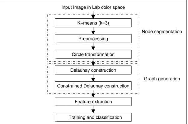
The proposed method comprises a series of processing steps. In the first step, the pixels of the image are clustered into three groups which correspond to nuclei, cytoplasm, and white (including lumen) areas using the k-means clustering algorithm. After a slight preprocessing is applied, the following step fits circular objects into these enclosed spaces of white areas and nuclei pixels with the help of circle-fit transform. The outcome constitutes the input, white and purple nodes, to the next step. Afterwards, a Delaunay triangulation is built on the set of nodes initially. A graph is constructed out of the initial triangulation with the use of our novel constraint definition on constrained Delaunay triangulation, and various features are extracted from this resulting graph. Finally, training
and classification of the images is accomplished by using these feature sets. The overall system architecture is shown in Figure 3.1.
Input Image in Lab color space
Node segmentation K−means (k=3) Preprocessing Circle transformation Graph generation Delaunay construction
Constrained Delaunay construction
Feature extraction
Training and classification
Figure 3.1: Overall system architecture
As demonstrated in Figure 3.1, the system architecture consists of four main components: Node segmentation, graph generation, feature extraction, and classification. Details of these components are given in the rest of this chapter. Throughout these sections, biopsy images shown in Figures 3.2a, 3.2b, and 3.2c will be used to demonstrate the output of the corresponding step. They are the images of the tissues that are healthy, low-grade cancerous, and high-grade cancerous, respectively.
3.1
Node Segmentation
Increasing the accuracy of diagnosis and grading in graph-based approaches is directly concerned with proper positioning of nodes. High-quality node segmen-tation results in a more representative graph which reflects the architecture of
(a) Healthy
(b) Low-grade cancerous
(c) High-grade cancerous
the tissue it is built on better. It also reduces the effects of artifacts, noise, and color variation due to hematoxylin-and-eosin (H&E) staining. In our problem, for colon tissues stained with the H&E staining technique, it may sometimes be impossible to cope with indistinguishability of nuclei from each other. Besides, we also need symbolic white nodes which will represent the lumen structures. For the node segmentation problem, we follow the steps whose details are given below.
3.1.1
Transforming into Lab color space
Lab color space is a color-opponent space, which is originally aforethought to estimate cognitive vision of homogeneity of human. The color space, with the components L for lightness, a and b for the color-opponent dimensions, improves the computerized image analysis methods with its L component closely matching human perception of lightness [53].
The segmentation component of our system first transforms the RGB biopsy images to Lab color space for the histopathological analysis. The intent was to simulate human perception of color at first, and later experiments proved the advantages of the use of Lab color space over RGB color space, and more accurate segmentation is provided by this color space.
3.1.2
K-means clustering
The well known k-means clustering algorithm is a process to partition N-dimensional population into k sets and it has been one of the simplest unsuper-vised learning algorithms [79]. The algorithm attempts to locate cluster centers of k sets by minimizing the sum of distances over all clusters, where different distance approaches are proposed. Basically, the sum of squared Euclidean dis-tances from points to cluster centroids is accepted as the distance function in our system. With k being the desired number of clusters; Si, i = 1, 2, . . . , k being the
the distance function: D = k X i=1 X xj∈Si (xj− µi)2 (3.1)
The k-means algorithm is useful to discriminate the white, nuclei and cytoplas-mic regions’ pixels of the biopsy images. In our problem, the k-means algorithm is applied on the images with k = 3 to differentiate these three disjoint regions. Right after detecting which pixels belong to which regions, average L values of the regions are used to determine the type of cluster vectors (white, nuclei or cytoplasm). In Lab color space, L represents the lightness of color, which yields 0 for black and 100 for diffuse white. Hence, the cluster vector with the highest L value, and its corresponding pixels can be labeled as white and the darkest one and its corresponding pixels can be labeled as nucleus, leaving the remaining one left and its pixels as cytoplasm, which has a pink color in RGB space.
It is observed that selecting k value as 3 is adequate and sufficient for our problem, because the H&E staining technique dyes chromatin-rich nuclei regions with dark purple, eosinophilic cytoplasm regions (belonging to stromal cells and connective tissues) with pink, and releases the vacant regions as it is, white. Consequently, the k-means algorithm easily recognizes and distinguishes pixels of three dissimilar zones in the image, and Lab conversion also increases the rate of separation. The clustered output of the k-means algorithm for the sample tissue images (Figure 3.2) are presented in Figure 3.3.
3.1.3
Preprocessing
After k-means clustering, we have labeled maps (pixels), which have noise on a small scale. To eliminate noise, we have preprocessed these maps and applied some morphological operations. These operations include a morphological close operation followed by a morphological open operation with a flat, square struc-turing element with edge length of 3 (for the histopathological images at the resolution 640 × 480). Close operation removes small gaps and eliminates noisy
(a) Healthy
(b) Low-grade cancerous
(c) High-grade cancerous
data, while open operation disqualifies the undesired results of close operation, turning the regions back into their original penetration and scope.
3.1.4
Circle-fit transform
With the execution of the k-means clustering algorithm and preprocessing step, the pixels of the original image are classified and appointed to the correct pixel group. Although the pixel classification provides the essential information about tissue distribution, the outcome itself does not contribute to nuclei and lumen segmentation. The reason is that, given earlier in Section 1.1, the boundaries of individual nuclei of colon tissues are occasionally uncertain and they are even inseparable to the experienced specialists’ eye. An alternative segmentation and node definition algorithm, which better suits the needs of segmentation of colon tissues, should be applied to eliminate the necessity of a high-quality segmenta-tion.
In literature, there exist some studies which split the segmentation problem into subproblems covering the nucleus segmentation, luminal region segmentation and epithelial cytoplasm segmentation, and then unify the solutions altogether to create a unique, segmented tissue image [82, 91, 92]. However, this approach put forwards the problematic nature of segmentation. They also require high-magnification biopsy images or high-dimensional hyperspectral data. Besides, according to our present knowledge, there do not exist any studies on cytoplasm and lumen segmentation.
From another perspective, the solution to the node segmentation problem might turn into decomposing the clustered image into a series of connected com-ponents and using each individual connected component as a separate node. How-ever, our experiments have shown that this methodology results in a significant decrease in classification quality, because of the aforementioned reasons.
To overcome all these problems, we have decided not to segment each actual individual histological component, but approximately represent them. For this
purpose, we have made use of a technique called circle-fit transform, which fits the largest circles available into the given connected components. The algorithm of circle-fit transform is detailed in [71, 115].
The motivation behind the use of circle-fit transform is that cell nuclei gen-erally have globular forms, and appear circular in two dimensional microscope scanning. These entities are represented by a single circle in the resulting map of circle-fit transform. On the other hand, wide lumen areas are represented by a single large circle, and/or a few smaller circles inside the luminal area. The circle-fit algorithm removes the circles with a radius below a certain predefined threshold, therefore, this scheme gives rise to the elimination of the artifacts. Epithelial cytoplasms are usually transformed into medium-sized circles around lumen circles, however, the rest of our methodology does not require this distinc-tion. Henceforth, the circles fitted into nuclei regions are referred to as purple circles, and those which are fitted into luminal or arbitrary vacant regions around or inbetween gland bodies or epithelial cell cytoplasms are referred to as white circles. Fitted circles for the previous sample tissues in Figure 3.2 are presented in Figure 3.4, where cyan circles corresponds to the white circles.
Having two distinct types of nodes, purple circles and white circles, we may utilize these circles as nodes to enhance the graph generation algorithms. In the next section, we will be discussing the details of our graph generation approach.
3.2
Graph Generation
The center of the fitted circles release the coordinates of nodes in two dimensional space, on which we will build our novel graph, constrained Delaunay triangula-tion. In this section, we will first define the conventional Delaunay triangulation on the set of nodes which reside at the middle of white circles and purple cir-cles, white nodes and purple nodes, respectively. Afterwards, we will explain the details of the mechanism that vitalizes the constrained Delaunay triangulation.
(a) Healthy
(b) Low-grade cancerous
(c) High-grade cancerous
3.2.1
Delaunay triangulation
In previous studies (see Section 2.2.2), Delaunay triangulation algorithm is exten-sively used for the characterization and description of the tissue. Those studies used Delaunay triangulation, which is built on a set of nodes that represent nu-clei of cells in the tissue for the favor of histopathological analysis. The reason behind is that Delaunay triangulation carries the required characteristics which reflects the structuring of the tissue it is built on better than some of the other graph types. Another reason is that the generality of the Delaunay triangulation shall provide the fundamental skeleton to the other types of graph. For exam-ple, a minimum spanning tree of a set of points P is a subgraph of Delaunay triangulation of P .
These former approaches have been beneficial for tissues without dominant hierarchical structures and have provided a distinctive set of features that in-creases the diagnosis and grading accuracy. However, not every tissue is plain as those like liver or lymph node tissues. For the tissues with hierarchical structures such as colon tissues with gland structures, these approaches are insufficient in recognizing such structuring of the tissue on its entirety. Presented in Figure 3.5, the outcome is not that representative enough to analyze the status of glandular structures.
As a solution to this problem, one may think of utilizing the representative nodes we have defined on the other tissue components, as explained in the pre-vious section. For this purpose, we first form a Delaunay triangulation on the set of nodes composed of purple nodes and white nodes. The formal definition of this Delaunay triangulation is given as follows:
Definition 5 Let Sp be the finite set of primary nodes and Ss be the finite set of secondary nodes. Non-collinear points pi, pj and pk of set Sw∪ Sp form a Delaunay triangle t if and only if there exists a location x which is equally close to pi, pj and pk and closer to pi, pj, pk than any other pm ∈ Sw∪ Sp. The location x is the center of a circle which passes through the points pi, pj, pk and contains no other points pm of P. For the 2D space, there exists only one circle, which is
(a) Healthy
(b) Low-grade cancerous
(c) High-grade cancerous