Effective Heuristics and a Cycle Time Minimization Procedure
Selcuk Karabati"
Bilkent University, Management Department, Faculty of Business Administration, Bilkent, Ankara 06533, Turkey
Panagiotis Kouvelis
Duke University, The Fugua School of Business, Durham, North Carolina 27708
In this paper we address the cyclic scheduling problem in flow lines. We develop a modeling framework and an integer programming formulation of the problem. We subsequently present exact and approximate solution procedures. The exact solution procedure is a branch-and-bound algorithm which uses Lagrangian and station-based relaxations of the integer programming formulation of the problem as the lower bounding method. Our heu- ristic procedures show a performance superior to the available ones in the literature. Finally, we address the stability issue in cyclic scheduling, demonstrate its relationship to the work- in-progress inventory control of a flow line, and present a very simple procedure to generate stable schedules in flow lines. 0 1996 John Wiley & Sons, Inc.
1. INTRODUCTION
In this paper we address the cyclic scheduling problem of a flow line with the perfor- mance objective of maximizing the throughput rate of the line. Some of the advantages of cyclic scheduling policies over conventional scheduling techniques for current flow line environments are mentioned in the research literature (Matsuo [ 121, Lee and Posner [ 91) and include benefits such as better station utilization, smoother finished goods inventory levels, and implementation convenience due to the simplicity of cyclic schedules.
The operating environment of a flow line under a cyclic scheduling policy can be de- scribed as follows. The system consists of
m
stations in series with finite or infinite capacity buffers between the stations. Let rl be the number of units of itemI,
1 = 1,2,.
.
.
, L, required to meet a production target of the line over a planning horizon, and r = ( rl,
. . .
, rL ) be the production requirement vector. If q is the greatest common divisor of integers rI ,. . .
, rL, then the vectorr* =
( 3 ,
. . .
,:)
9
is referred to as the Minimal Part Set (MPS) (term introduced by Hitz [ 81). It represents the smallest part set having the same proportions as the production requirement vector.
*
Current address: College of Administrative Sciences and Economics, KO$ University, Cayir Cad. No. 5, Istinye, Istanbul, 80860, TurkeyNaval Research Logistics, Vol. 43, pp. 2 I 1-23 1 ( 1996)
Under a cyclic scheduling policy, the flow line will produce an integral multiple of MPSs. A part set that is an integral multiple of MPS is represented through its production re- quirement vector
where a is an integral constant of proportionality and a divisor of q . The above part set is referred to as the a-multiple MPS (a-MPS). In our analyzed flow line environment the processing times of the various items are assumed to be known and deterministic. Note that an MPS (or a-MPS) contains more than one unit of item I, when r / / q > 1, I = 1, 2,
. . .
,
L . However, each element of the MPS represents a job to be processed by the system, and our scheduling task is to sequence these jobs. We treat every element of the MPS as an individual job, although some of these jobs may belong to the same item group. Therefore, the total number of jobs in an MPS is equal to n = Ck,
r / / q . We denote by p o , i = 1,. . .
, n , j = 1,. . .
, m , the processing time of job i on station j . Then our cyclic scheduling problem is to find the optimal sequence of jobs in a prespecified part set (i.e., a-MPS for a given a 2 1 ) in order to optimize the throughput rate of the line, or equivalently its cycletime (i.e., the reciprocal of the throughput rate of the line). We are restricting our analysis to the operation of conventional flow lines (i.e., by-passing of stations by some jobs is not allowed). For references on flexible flow lines, which allow station by-passing by some jobs, see Hitz [ 81 and Wittrock [ 201.
The cyclic scheduling problem for flow lines has been recently studied in some detail. McCormick et al. [ 141 established the computational complexity of the problem. The cy- clic scheduling problem for cycle time minimization is unary NP-complete for arbitrary processing times. A polynomial time algorithm for a special case of the problem has been presented by Matsuo [ 121. He analyzed the two station flow line with a zero capacity buffer between the stations. McCormick et al. [ 131 have presented a heuristic solution procedure for the problem.
The cyclic scheduling problem has been discussed in various settings. Bartholdi [ 11 has addressed the problem of cyclic staff scheduling and presented a heuristic solution proce- dure. Graves et al. [ 61 address the scheduling problem in a reentrant flow shop, and present a heuristic solution procedure for the problem. In Hall [ 71, the notion of cyclic production scheduling approach and its benefits have been discussed in detail. Roundy [ 18 ] addresses the cyclic scheduling problem in a job shop with identical jobs. Cyclic scheduling of a material handling network has been discussed in Lei and Wang [ 101. Bowman and Muck- stadt [ 21 address the cyclic scheduling of operations in a multi-machine environment, and analyze the performance of cyclic schedules under stochastic variability in processing times. Dauscha et al. [ 31 discuss the problem of cycling scheduling of a finite set of tasks, prove an existence criterion for cyclic schedules, and investigate some complexity issues in cyclic scheduling. Whybark [ 191 describes an actual production planning and control sys- tem which is an implementation of the cyclic scheduling approach. In Rao [ 161 the iden- tical jobs, single end-item cyclic scheduling problem is addressed, and a set of sequencing heuristics is developed and tested. Rao and Jackson [ 17 ] study two subproblems that are encountered in the identical jobs, reentrant flow cyclic scheduling problem. Fuxman [ 41 studies the team organization of workers in mixed-model assembly lines under cyclic pro- duction. Loerch and Muckstadt [ I 11 address the cyclic production planning and schedul- ing problem.
In this paper we develop an integer programming formulation of the cyclic scheduling problem in flow lines. Our optimal procedure for the above formulation is a branch-and- bound approach, and can handle cycling scheduling of 12 jobs per MPS and up to ten stations for various buffer configurations between the stations. For larger size problems we propose two new approximate solution procedures. One of the approximate solution procedures is a simple constructive heuristic, while the other one is based on an early ter- mination of the branch-and-bound procedure. Both heuristic procedures outperform the best available in the literature (see McCormick et al. [ 13 ] ).
In the cyclic scheduling literature the concept of stability of schedules plays an important role. For a detailed reference on this concept see Lee and Posner [ 91. The authors discuss the concept in a general job shop environment with infinite capacity buffers, and present a graph theoretic framework for stable schedule generation. In flow lines the stability of a schedule is directly related to maintaining low work-in-progress ( WIP) inventory levels, as we will further discuss later. Another research contribution of our paper is the development of a simple way to generate stable schedules in a flow line environment.
The structure of the paper is the following. In Section 2 we discuss a graph theoretic modeling framework of job completion times in cyclic scheduling flow line environments. Building on the previous modeling framework, in Section 3 we present a formal statement of the cyclic scheduling problem as an integer program. Section 4 discusses the use of relaxation approaches for lower and upper bound generation on the optimal cycle time values of cyclic scheduling problems. Section 4 constitutes the backbone of the branch- and-bound procedure suggested for the optimal solution of the problem. The details of the procedure, as well as our computational experience with it, are presented in Section 5 . For the solution of large size problems we suggest the use of heuristic solution procedures whose details and successful performance are documented in Section 6. A stable schedule gener- ation scheme for flow line environments is discussed in Section 7. Section 8 concludes the paper with a summary of our results.
2. A MODELING FRAMEWORK FOR THE CYCLE TIME CRITERION
For the production environment described in Section 1, let us consider the operation of the line under the cyclic scheduling approach. The jobs of an MPS (or a-MPS) go through the system in a given order followed by a second MPS (or a second a-MPS) in the same order and so on. A total of q (or q / a ) runs of an MPS (or a-MPS) is required to meet the production target of the line over the planning horizon. Our discussion below concentrates on sequencing jobs of an MPS, however, the same approach can be readily extended to sequencing jobs of an a-MPS.
An MPS schedule will be represented by permutation a = ( a( 1 ), a( 2 ) ,
.
. .
,
a( n)) where n is the number ofjobs in the MPS and a( i) is the ith job in the processing order. Note that we restrict our analysis to permutation schedules only, i.e., no job passing is allowed once the MPS is released to the system. Job a( i) in the rth MPS is said to be the rth repetition of job a( i) and is denoted by a,( i).McCormick et al. [ 131 have shown that a unit capacity buffer can be represented as a station at which the processing times of all jobs are equal to zero. Therefore, without any loss of generality, we may assume that all buffers have either zero or infinite capacity, because a finite capacity buffer can be represented as a series of unit capacity buffers. This transformation increases the number of stations in our problem, however, as we will dem-
1st MPS
2nd MPS
Figure I .
onstrate later, it does not increase the computational effort required by our optimal solu- tion procedure for the minimum cycle time problem.
Let us consider a flow line with zero capacity buffers. The completion time C( a,( i), j )
ofjob a,( i) on station j can be found using the following recursive relationship:
This recursive relationship can be represented by the directed graph presented in Figure 1. Vertices ( a,( i ) , j ) are defined for each element a( i) of the permutation, for r = 1, 2,
. .
.
, and each station j . Directed arcs are defined from each vertex (a,( i), j ) towards vertices (a,( i+
1 ) , j ) , ( a,( i ) , j+
1 ) and ( u,( i+
1 ) , j - 1 ), where C( a1 ( O ) , j ) = 0 , j = 1,2,. . .
, m , C(a,(i),O)=O,rr l , i = 1,2,...,
n , a , ( O ) = ~ , - ~ ( n ) , r > I , a nda, ( n+ l ) = ~ , + ~ ( l ) , r z 1, due to the cyclic nature of the problem. The directed arc from vertex (a,( i ) , j ) to vertex ( a,( i+
1 ), j - 1 ) accounts for the blocking of jobs due to the zero capacity buffer between stations j - 1 and j , and therefore should be removed from the graph if there exists an infinite capacity buffer between stationsj - 1 andj. A weight p d i ) , is associated with vertex ( a,( i), j ) , if the vertex is entered via either the horizontal or the vertical directed arc that are adjacent to vertex (a,( i ) , j ) . We note that when an operation is blocked, i.e., the cor- responding vertex is entered via the diagonal directed arc, its processing time does not affect its completion time, and therefore the weight of the vertex is set equal to zero.Figure 2.
is equal to the weight of the maximum-weighted directed path from ( a1 ( 1 ), 1 ) to (a,( i), j) in the graph, as follows immediately from the recursive relationship ( 1 ).
The performance criterion we want to optimize is the throughput rate of the flow line, or equivalently its cycle time. To define the cycle time of a flow line in our modeling frame- work, we need to introduce the notion of a cylinder formed by the directed graph of a single MPS, which is depicted in Figure 2. Therelationship of the cycle time to the above concept comes from the following theorem:
THEOREM 1: (McCormick et al. [13]) The weight of the maximum-weighted path around a cylinder formed by the directed graph of a single MPS equals the cycle time.
Our representation of the MPS cylinder is slightly different than that of McCormick et al.’s, in our cylinder the processing times are represented as vertex weights instead of arc weights. This approach is necessitated by our formulation of the cyclic scheduling problem. We now introduce a convenient way of computing the weight of a path around the cylinder. Let T be a path around the cylinder, i.e., a chain of vertices that starts at a partic-
ular vertex and ends at the same vertex after completing one tour around the cylinder. We note that in a given tour around the cylinder no vertex is visited more than once, because the directed graph is planar and contains no sub-tours. Let
w;,
i = 1 ,. . .
,
n, be the station index of the right-most operation ofjob a( i) on path T . We have the following property:w;- 1s w ; , and w k l - 1 s w;, i = 2 , 3 , .
. .
, n ,with the equality holding if job a( i) is blocked on station wT by job a( i - 1 ) on the tour defined by path T (i.e., vertex (a( i),
w;)
is entered via vertex (a( i - 1 ), wTPl), where w;-,= w ;
+
1 ). It follows that pdi),k is included in the weight of path T if and only if w ; - ~ 5 k Iwl.
Letf( a, T ) be the weight of path T , when the cylinder is formed using the permutationFor any given path 7 E T , we can determine the unique set of integers W' = ( 1 I w ; I rn, i
= 1,2,
.
. .
, n ) to represent the weight of the path using the above functional form.We will illustrate the characterization of a path by a set of integers using the following example.
EXAMPLE I: Consider a three jobs per MPS three station problem where the buffer capacity between stations 1 and 2 is infinitely large and the buffer capacity between stations 2 and 3 is zero. The cylinder of this problem is presented in Figure 3. The path T is given
by the dark lines in Figure 3. Now the weight of path 7 is equal to
We note that operation (a( 2 ) , 2 ) is blocked by operation (a( 1 ), 3 ) and therefore P , , ( ~ ) , ~ is not included inf( u, T ) . The right-most operation of a( 1 ) on path T is (a( I ) , 3 ) , therefore
w ; = 3. Similarly, wl = 2, and w ; = 2. Now, let w' = ( 3 , 2 , 2 ) , then
3 2 2
f(a,T)'
2
P d l ) , k +c
P u ( 2 ) , k +2
P u ( ~ ) , ~ = ( P ~ ( I ) , ~ + P u ( I ) , ~ ) + ( ~ ) + ( P u ( ~ ) , ~ ) . k=2 k = 3 k = 2The representation off( u, 7 ) in the above functional form will play an important role in the
development of an integer programming formulation for the cyclic scheduling problem. 3. AN INTEGER PROGRAMMING FORMULATION OF THE MINIMUM
In this section we present a modeling framework for the minimum cycle time problem. In developing our framework we will use Theorem 1 in Section 2. Theorem 1 states that
the weight of the maximum-weighted path around a cylinder formed by a single MPS equals the cycle time. Let T be a path around the cylinder as depicted in Figure 2, and T be
the set of all paths around the cylinder. We note that the elements of set Tare independent of the sequence of jobs, i.e., the structure of the cylinder is the same for all permutation sequences, only the vertex weights are affected by the sequence of jobs. We denote byf( u,
T) the weight ofpath T E Twhen the cylinder is formed (i.e., vertex weights are determined)
using MPS schedule u. Let A, denote the cycle time of this schedule. Then A, is given by A, = maxf( u, T )
7 € T
If we let S be the set of all MPS schedules, the minimum cycle time problem can be for- mulated as
A* = min maxf( u, T ) ,
rnS r E T ( 3 )
and A* is the optimal cycle time for the problem. In the rest of the paper we will use the abbreviation n / m / P , D / h for the minimum cycle time problem with n jobs per MPS, m stations, and buffer configuration D. The buffer configuration indicates the number of buffers between adjacent stations. For example, for m = 4,
D
= (2, 1,2) describes a buffer configuration with two unit capacity buffers between the first and second stations, one unit capacity buffer between the second and third stations, and two unit capacity buffers be- tween the third and fourth stations. The symbol P reminds us of our restricted attention to permutation MPS schedules, and A refers to the cycle time criterion.Using the above established modeling framework, we can now state the following prop- osition.
PROPOSITION 1 :
max minf( u, T ) I min maxf( u, T ).
s€T &S &S r E T ( 4 )
PROOF: Let uo E S be a specific MPS schedule and T~ E Tbe a path around the cylinder.
Then
However, ( 5 ) holds for every uo E S and T~ E T, therefore the validity of (4) follows im-
mediately. 0
Proposition 1 states that for any path around the cylinder, T E T, the solution to the
optimization problem
(AP,): minf( u, T )
CTES
provides a lower bound for the problem as formulated in ( 3). Some further insight on the nature of ( A P , ) is provided by the following result.
PROPOSITION 2: (AP,) is equivalent to a linear assignment problem.
PROOF According to (2), for a specific path 7 E T, there exists a unique set of integers wT = ( w ; , w ; ,
. . .
, w ; ) such that for any u E S , we have the following:where 1 { } is an indicator function and w & = w ; . Let us denote by
Then ( 6 ) can be rewritten as
Using relationship ( 7 ) one can easily observe that ( A P T ) is equivalent to a linear assignment problem with cost matrix A' = ( a
;,
j ) . 0We can write an integer programming formulation of the cyclic scheduling problem as follows: We first introduce the set of binary decision variables
xij
E { 0, 1 },
to equivalently describe a schedule as( u E S )
-x
= (Xi,.),where
1, if u(j ) = i, 0, otherwise.
Using the above set of decision variables and relationship ( 7 ) we can state the problem in an equivalent way as follows:
( I P ) :
f
*
= min Msubject to
n
C X i , j = l , j = 1 ,
. . . ,
n, i= In
C x i , , = l , i = l ,
...,
n ,j = I
x ; , ~ E { O , l}, i , j = 1
,...
, n . ( 1 1 ) In the next section we present a lower bounding scheme for then / m / P ,
D / h problem which is based on a relaxation of formulation(IP)
.
4. A LOWER BOUND GENERATION SCHEME FOR THE n / m / P , D/X PROBLEM '
In order to develop lower bounds for the
n/m/P,
D/X problem, we are going to use a relaxation of formulation(ZP).
In the relaxed problem, we restrict our attention only to a subset T* of the path set T. The relaxed formulation of(IP)
is given as follows:(RIP):
f = min M subject to(9), ( 10) and ( 1 1 ).
We now present two lower bounding procedures based on formulation
(RIP).
4.1. The Lagrangian Relaxation Lower BoundIn our first lower bounding approach, we dualize the constraint set ( 1 2 ) . Let p = { p, 2 0,7 E T* } be a set of Lagrange multipliers. Then, the Lagrangian relaxation of
(RIP)
issubject to ( 9 ) , ( 10) and( 1 1 ) .
Observe that f ( p ) is bounded only if
CrET*
p, = 1. Without loss of generality, we can always assume that this is the case, since we can normalize the Lagrange multipliers p T , 7E T*, by their sum
C r E P
p,. Therefore, we can always state ( L R ( p ) ) as an equivalent linear assignment problem as follows:subject to (9), ( 10) and ( 1 1 ).
Let
f
:'be the optimal objective function value of the linear programming relaxation of(RIP).
Let Q = { p €RIPl
I
Z r E p p L , = 1 andpL, 2 0,7 € T*} beaset ofmultipliervectors.Using standard results from the Lagrangian relaxation theory (see Nemhauser and Wolsey [ 15 ] ), we can state the following property.
PROPERTY 1 :
From our above discussion, we can conclude that
f
T
is a legitimate lower bound for the n / m / P , D/X problem, i.e.,f ~f
*.
We can always approximatef?
from below by solv- ing the linear programming relaxation of (RIP). From well known results of Lagrangian relaxation theory, and since the constraint set of (LRAP( p ) ) has a network structure, we are guaranteed that our Lagrangian bound cannot be better than the linear programming relaxation bound. The solution of the linear programming relaxation of(RIP),
however, proved to be computationally prohibitive when we implemented it within a branch-and- bound approach. Thus, we decided to use a slightly different approach. To obtain ff.',
or a lower bound on it, we solve the linear assignment problem (LRAP( p ) ) for an appropri- ately chosen vector p E Q. The use of a subgradient optimization method helps us update the multiplier vector 1.1, and within a small number of iterations generates a very good approximation off f.'. Our subgradient optimization procedure starts with an initial mul- tiplier vector po Ea,
and then defines iteratively a sequence of multiplier vectors p' by use of the following rulewhere p' is a scalar, f-is an upper bound on
f
f-', ( = ( f7, T E T*) is a subgradient for& ( P I ) , and llpll is the Euclidean norm of the vector p. The notation
if
=(ji:,
T E T*)denotes the multiplier vector before the required normalization procedure for our method. The above subgradient optimization procedure is an adaptation of the one presented in Goffin [ 5
1,
and based on results therein it is guaranteed to converge tof
f.',
whenC
Fo
p' = 00 and limf+mp'
= 0. For the complete specification of the above procedure we need to describe the subgradient vector {. This is described in Property 2 below.PROPERTY 2: Let
L
=C6,
Cy=,
aTjx?' - h P ( p ) , T E T*, whereX*
= (x?') is the optimal solution to the ( L R A P ( p ) ) problem. Then, { = (Cr,
T E T*) is a subgradient for f A P ( P ) .PROOF: We present the proof of Property 2 in Appendix A.
4.2. The Contiguous Stations Lower Bound
For flow lines with at least two contiguous stations, i.e., two stations with a zero capacity buffer in between them, a station-based, and potentially tighter, lower bounding procedure can be developed based on formulation (RIP). In formulation (RIP) we use a subset T* of the path set T. L e t j a n d j
+
1 be two contiguous stations, and T* be the set of paths around the cylinder formed by stations j and j+
1. Now(RIP)
is equivalent to a two station, zero capacity buffer problem which can be solved in O ( n log n ) time (Matsuo [ 121). Therefore, in flow lines with contiguous stations the above described procedure can be used to develop lower bounds for the minimum cycle time problem, because, as we havediscussed earlier, the optimal value
f
T
of formulation ( R I P ) constitutes a lower bound for the original problem.We have used these lower bound generation schemes within a branch-and-bound algo- rithm. We will discuss the implementation and quality of the new bounding techniques in the next section.
5. A BRANCH-AND-BOUND ALGORITHM
In this section we present an optimal algorithm for the n / m / P , D / X problem and report on our computational experience with the algorithm.
5.1. Description of the Algorithm Our branching and bounding schemes are as follows:
Branching Scheme: The branching scheme used in our solution procedure defines the nodes of the search tree as partial schedules. A node at the kth level of the search tree corresponds to a partial schedule of size k, i.e., a schedule where assignments are made to the first k positions. When branching from a node of the search tree at the kth level, we create ( n - k) nodes at the ( k
+
1 )-st level by appending each unassigned job of the node to the end of the partial schedule of size k.Note that in our branching scheme we have assumed that MPSs are formed of noniden- tical jobs. However, when there are some identical jobs in the MPS, in order to decrease the size of the search tree, the above branching scheme can be modified to account for these similarities.
Bounding Scheme: In writing relaxation
(RIP)
for development of the Lagrangian lower bound, we choose1
T*I
paths around the MPS cylinder. In the current version of the algorithm,I
T*1
is created as follows: First we randomly create a permutation schedule, and determine its maximum-weighted path (see Section 2 for the determination of the maximum-weighted path). This path is then included inI
T*I.
Next, we solve (AP,) (see Section 3) on this path to generate another schedule. We then determine the maximum- weighted path of the new schedule, and include it inI
T*I.
We continue by solving (AP,)on this new path to generate a new schedule. This procedure is repeated until
I
T*I
reaches the required size. If a newly generated path is already inI
T*1,
the procedure is restarted with another randomly created schedule. In the current version of the algorithm we use 10 paths to obtain the Lagrangian lower bounds.The selection of paths is performed at the initial node of the search tree. However, as we move down in the search tree the size of the partial schedule (i.e., the number of fixed jobs) that corresponds to a particular node increases, and the set T* is modified so that the selected paths attain their maximum possible values on these partial schedules. This is accomplished by determining the maximum-weighted paths on the MPS cylinder’s fixed part, i.e., the part of the MPS cylinder that corresponds to the partial schedule of the node under consideration. These paths are later appended to the paths chosen at the initial node of the search tree.
The performance of our algorithm is very much affected by the selection of the initial multiplier vector j.t in the subgradient optimization method. Due to the above mentioned
selection of T*, the paths of a node and its immediate descendant nodes are very similar, and in most cases the multiplier vector obtained in the last iteration of the subgradient
method is a very good initial multiplier vector for the immediate descendant nodes of this particular node. In the current version of the algorithm, at each node of the search tree multipliers are updated four times, except the initial node where we iterate 20 times to obtain the initial multipliers.
We have used the alternative contiguous stations-based lower bounding procedure de- scribed in Section 4.2, along with the subgradient method, when the flow line under con- sideration has pairs of contiguous stations. In this case, the lower bounds generated by the station-based procedure are usually better than the bounds obtained using the subgradient method, due to the fact that in this approach (RIP) is directly solved without resorting to a further relaxation.
We also note that both lower bounding procedures generate complete schedules in de- veloping the lower bounds, and these schedules are evaluated for their cycle times to update the upper bound on the optimal cycle time value of the problem. However, the upper bounds generated by the subgradient method have dominated the upper bounds obtained by the contiguous stations-based procedure. This is due to the fact that the contiguous stations-based lower bounding procedure uses local information, i.e., only the processing times of the two contiguous stations, whereas the subgradient method considers the flow line in its entirety. Therefore we have decided to use these two bounding schemes concur- rently. Note that, if the flow line does not possess any contiguous stations, the contiguous stations-based procedure cannot be employed and the subgradient method becomes the only possible approach to generate lower bounds.
Fathoming Criterion: If the current upper bound is less than or equal to the lower bound on that subset of schedules.
Node to Examine Next Criterion: In the current version of our algorithm we examine next the subset of schedules that has the smallest lower bound.
5.2. Computational Results
We have tested the performance of the branch-and-bound procedure described in Sec- tion 5.1 using two sets of problems. The first set of test problems is the five problems with eight jobs per MPS and nine stations given in McCormick et al. [ 131. Our optimal solution procedure solved these problems with an average of 32.6 nodes and 0.19 CPU seconds per problem, on a multi-user IBM 308 1-D system. We also note that three of these test prob- lems have some identical jobs and the performance of our approach can be improved by taking the similarity ofjobs into account when branching in the search tree.
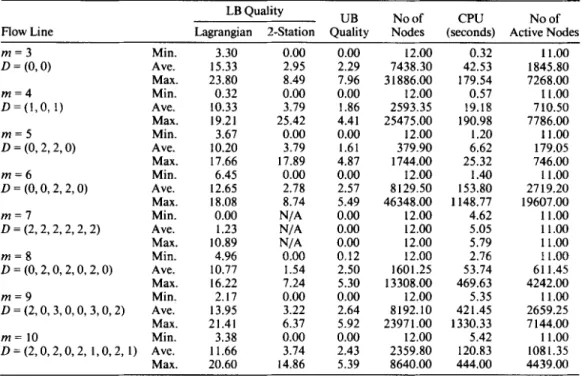
The second set of test problems is created using integer processing times drawn from a ( 1-100) uniform distribution. We have tested the performance of the algorithm for prob- lems with 12 nonidentical jobs per MPS. In Table 1, the first column documents the con- figuration of the line. For each configuration we created 20 problems. In Columns 3 and 4 of Table 1 , we present the minimum, average, and maximum difference between the lower bound value of the initial node of the search tree and the optimal cycle time value as a percentage of the optimal cycle time value, for the Lagrangian relaxation and contiguous stations lower bounds, respectively. In Column 5 of Table 1 , we present the minimum, average, and maximum difference between the upper bound value of the initial node of the search tree and the optimal cycle time value, as a percentage of the optimal cycle time value. Upper bounds are generated using the LIST heuristic which will be described in Section 6. Columns 6 and 7 of Table 1 tabulate the minimum, average, and maximum number of nodes and CPU times, respectively. Column 8 documents the maximum num-
Table 1. Performance ofthe branch-and-bound algorithm for 12 jobs per MPS problems. UB N o o f CPU No of LB Quality
Flow Line Lagrangian 2-Station Quality Nodes (seconds) Active Nodes m = 3 D = (0,O) m = 4 D = ( I , O , 1) m = 5 D = (0,2,2,0) m = 6 D = (0, 0 , 2 , 2 , 0 ) m = 7 D = (2,2,2,2,2,2) m = 8 D = ( 0 , 2 , 0 , 2 , 0 , 2 , 0 ) m = 9 D = (2,0, 3,0,0,3,0,2) m = 10 D = ( 2 , 0 , 2 , 0 , 2 , 1,0,2,1) Min. Ave. Max. Min. Ave. Max. Min. Ave. Max. Min. Ave. Max. Min. Ave. Max. Min. Ave. Max. Min. Ave. Max. Min. Ave. Max. 3.30 15.33 23.80 0.32 10.33 19.21 3.67 10.20 17.66 6.45 12.65 18.08 0.00 I .23 10.89 4.96 10.77 16.22 2.17 13.95 21.41 3.38 11.66 20.60 0.00 0.00 2.95 2.29 8.49 7.96 0.00 0.00 3.79 1.86 25.42 4.41 0.00 0.00 3.79 1.61 17.89 4.87 0.00 0.00 2.78 2.57 8.74 5.49 N/A 0.00 N/A 0.00 N/A 0.00 0.00 0.12 1.54 2.50 7.24 5.30 0.00 0.00 3.22 2.64 6.37 5.92 0.00 0.00 3.74 2.43 14.86 5.39 12.00 7438.30 3 1886.00 12.00 2593.35 25475.00 12.00 379.90 1744.00 12.00 8129.50 46348.00 12.00 12.00 12.00 12.00 1601.25 13308.00 12.00 8192.10 2397 1 .OO 12.00 2359.80 8640.00 0.32 42.53 179.54 0.57 19.18 190.98 1.20 6.62 25.32 1.40 153.80 1148.77 4.62 5.05 5.79 2.76 53.74 469.63 5.35 42 I .45 1330.33 5.42 120.83 444.00 11.00 1845.80 7268.00 11.00 7 10.50 7786.00 11.00 179.05 746.00 11.00 2719.20 19607.00 11.00 1 1
.oo
1 1.00 I 1.00 61 1.45 4242.00 11.00 2659.25 7 144.00 I 1.00 1081.35 44 39 .OOber of active nodes, i.e., nodes that have been stored for further branching during the im- plementation of the algorithm. The number of active nodes serves as an indicator of the storage requirements of the algorithm. Based on the results reported in Table 1, we can conclude that the algorithm exhibits a satisfactory performance over all tested problems. We also note that the contiguous stations-based lower bounds dominated the Lagrangian relaxation lower bounds in all of the test problems with contiguous stations.
The size of the problems solvable by the branch-and-bound procedure is limited by the number ofjobs which directly affects the size of the solution space, and the buffer config- uration ofthe flow line which largely determines the lower bound quality. The performance of the algorithm improves dramatically as the buffer sizes are increased. Therefore most difficult problems are those with contiguous stations. For n = 12, we were able to solve problems with twosomes of contiguous stations, provided that buffer sizes are greater than or equal to 2 between the groups of contiguous stations. Although it is very difficult to determine the limiting number of jobs without considering the buffer configuration of the flow line, for a limited buffers case, 12 seems to be largest number of jobs that can be efficiently handled by our procedure.
6. HEURISTIC SOLUTION PROCEDURES
As polynomial time algorithms are unlikely to exist for the n / r n / P , D/X problem, heu- ristic solution procedures are needed to obtain good schedules for large size problems. McCormick et al. [ 131 have developed a heuristic algorithm for cycle time minimization based on idle time and blocking time penalties. The McCormick et al. [ 131 heuristic can be described as follows: For a given partial sequence a penalty is computed for each un-
scheduled job. The penalty of a job is equal to the weighted sum of idle and blocking times caused by this job if it is appended to the end of the partial schedule. Then the job with the smallest penalty is assigned to the end of the partial schedule. The above step is repeated until the schedule is complete. McCormick et al. [ 13 ] have also observed that the heuristic that assigns more weight to idle time and blocking time on the bottleneck station performs better. In the rest of this section, we discuss two other effective heuristics for the cyclic scheduling problem.
The first approximate solution procedure we propose is a constructive heuristic. The heuristic starts with a partial MPS schedule of two jobs, along with a list of the remaining jobs. The first job on the list is used to create partial MPS schedules of size three, while keeping the relative positions of the first two jobs the same as in the partial MPS schedule. Among these newly formed partial schedules, we pick the one with the smallest cycle time. We then repeat the same procedure with an initial partial MPS schedule of three jobs and with the second job on the initial list. We repeat the same steps until all jobs are scheduled, i.e., we have a complete MPS schedule. The heuristic creates ;( n
+
1 )( n - 2 ) partial sched- ules, and for each partial schedule the cycle time can be computed inO(
nm2) time. There- fore the overall time complexity of the heuristic isO(
n3m2). The heuristic can be formally described as follows:Heuristic LIST:
Step 0: Let ?r = ( T ( 1 ), ?r( 2 ) ,
. . .
, T ( n ) ) be an initial sequence of jobs in an MPS.I n i t i a l i z e a ( l ) = ? r ( l ) , u ( 2 ) = T ( 2 ) a n d k = 3 . Step 1: For i = 1 to k
0 Set u , ( j ) = u ( j ) fo rj = 1,.
. . ,
i - 1, and i > 1.Set ui(i) =
~ ( k ) ,
and u , ( j ) = u ( j - 1 ) fo rj = i + 1,..
.
,
k.0 Compute the cycle time A; of partial schedule u;
.
Step 2: Let
I
= arg(minlshk A;). Set u ( j ) = q ( j ) , j = 1,. . .
, k.Set k = k
+
1, if k I n go to Step 1, otherwise stop, u is the resulting MPS schedule. Note that in the above heuristic procedure the initial sequence of jobs is an important input to the heuristic. We will use three different initial sequences.0 Jobs are sequenced according to nonincreasing total processing times (we refer 0 Jobs are sequenced randomly (referred to as LIST( umn)).
0 Jobs are sequenced according to non-decreasing total processing times
to this version of the heuristic as LIST( urnax)),
(referred to as LIST( urnin)),
Another alternative approximate solution procedure is the early termination of the branch- and-bound (B&B) algorithm. One of the advantages of our lower bounding scheme is that in the process of obtaining a lower bound we also obtain a feasible schedule, as we men- tioned in Section 4. We have used the best heuristic solution obtained as an initial upper bound for the B&B procedure and terminated the search after a prespecified number of
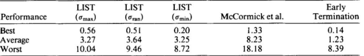
Table 2. Performance of heuristics for 20 jobs per MPS problems.
LIST LIST LIST Early
Performance (urnax) (Urn") (urnin) McCormick et al. Termination
Best 0.56 0.5 1 0.20 1.33 0.14
Average 3.27 3.64 3.25 8.23 1.23
Worst 10.04 9.46 8.72 18.18 8.39
nodes were generated in the search tree. The best lower bound obtained so far in the search tree was also used to measure the performance of the proposed heuristic procedures.
The experimental test bed for our heuristics is generated in the following way. We created random problems with 20 and 25 nonidentical jobs per MPS. The processing times of the various jobs on the different stations were drawn from a ( 1- 100) uniform distribution. The 20 jobs per MPS problems were tested on a flow line with eight stations and configuration
D
= (0, 0, 1, 0, 1, 0,O). We have experimented with 20 such random problems. The results are reported in Table 2. What we refer to as the performance of the heuristic is ( UB - LB/ L B ) X 100, where UB is the cycle time generated by the heuristic and LB is the best avail- able lower bound for the problem, as obtained from the early termination of the B&B procedure (after 500 nodes were generated in the search tree). The heuristics for which we are reporting results are the LIST( emax), LIST( bran), LIST( ernin), McCormick et al. [ 131,and the heuristic run of the B&B procedure. For the McCormick et al. [ 131 heuristic we used ten different combinations of idle and blocking time penalties and reported the best cycle time obtained by these combinations. The first row of Table 2 tabulates the best performance of these heuristics over the 20 random problems, the sec6nd row reports their average performances and finally the last row reports the worst exhibited performance of the heuristics. Our results for 25 jobs per MPS problems are reported in a similar manner in Table 3. We report results for 20 random problems nine stations and configuration
D
= ( 0, 2,0,0 , 1,
0, 1,O). A summary of the observed results is the following. For 20 (25 )jobs per MPS problems the average CPU time for the LIST heuristic (over all its variations) was 0.45 ( 1.47) CPU seconds. The variations of the LIST heuristic exhibited quite similar CPU requirements, and that was the main reason for averaging the CPU time over all of them. Our implementation of the McCormick et al. [ 13 ] heuristic had an average CPU time of 0.01 1 (0.023) seconds. The B&B procedure had an average CPU time of 6.20 ( 10.00) seconds, excluding the time spent to obtain the first upper bound, i.e., time spent for the LIST and McCormick heuristics. The results of Tables 2 and 3 indicate that the LIST heuristic clearly dominates the McCormick et al. [ 131 heuristic for any initial sequence selection. We note that the complexities of the McCormick et al. [ 131 and LIST heuristics are O( n2m) and O( n 3m2), respectively, and the improved performance is attained at the expense of larger run times. Among the LIST heuristic variations, the LIST( emin) and LIST( em") seem to dominate the LIST( urnax). The heuristic performance of the B&B pro-Table 3. Performance of heuristics for 25 jobs per MPS problems.
LIST LlST LIST Early
Performance (5rnw.) (5t-a") (5min) McCormick et al. Termination
Best 0.17 0.11 0.36 1.41 Average 2.98 2.63 2.66 7.76 Worst 9.56 8.82 10.25 17.21 0.1 1 1.35 7.97
cedure is very good, and though its computational burden is heavier, still it remains within a very reasonable range. Either the LIST or the heuristic execution of the B&B algorithm can be used effectively for large size real problems.
7. STABILITY OF CYCLIC SCHEDULES
In this section we address the concept of stability of cyclic schedules in flow lines, and present a simple procedure to generate stable schedules. As our discussion will show, the stability concept is closely related to the control of the WIP inventory levels of cyclic sched- ules, and thus the generation of stable schedules becomes an issue of importance for the scheduler. For example, two schedules having the same cycle time may have different WIP inventory levels in steady state, and our procedure can be used to determine the schedule having the smaller WIP inventory level in steady state without actually implementing the schedules. The control of the WIP level is of particular importance in flow lines with at least one infinite capacity buffer, where an earliest start schedule may result in unbounded WIP inventory levels.
First, we present a formal definition of stable cyclic schedules in flow lines following the work of Lee and Posner [ 91.
DEFINITION 1 : Let c be an MPS schedule and X be its cycle time. A schedule is periodic at ro if
for some integer d, i = 1,
. . .
, n, j = 1,.
. .
,
m and r 2 ro. When d = 1, such a schedule issaid to be stable at ro, In particular when d = 1 and ro = 1, such a schedule is simply said to be stable.
The following result of McCormick et al. [ 131 is important for our further discussion: THEOREM 2: ( McCormick et al. [ 131) Let c be an MPS schedule, and X be its cycle time. Then in a flow line with finite capacity buffers there always exists an integer k such that
for i = 1,
. . .
, n, a n d j = 1,. . .
, m , wherek
is finite.Theorem 2 guarantees that, in a flow line with blocking, i.e., with finite capacity buffers, every schedule becomes stable after a finite number of MPSs. Once the stable state is reached, we can compute the average WIP inventory level using Little’s formula:
1 X
WIP Inventory Level = - X (MPS Makespan) batches/unit time,
because in the stable state every MPS will have the same makespan or waiting time in the system. We note that the value of
k
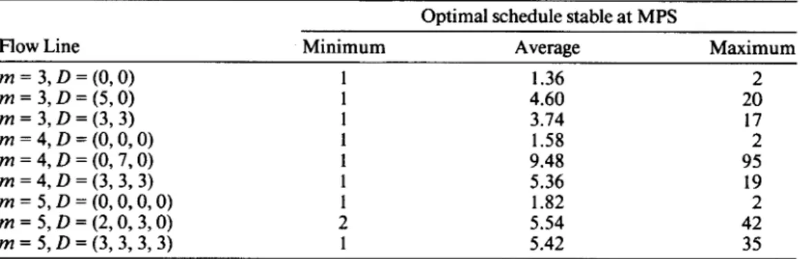
in Theorem 2 depends largely on the buffer configu-Table 4. Stability of optimal schedules.
Optimal schedule stable at MPS
Flow Line Minimum
m = 3, D = (0,O) m = 3, D = ( 5 , O ) m = 3, D = (3,3) m = 4, D = (0, 0,O) m = 4, D = (0,7,0) m = 4, D = (3,3,3) m = 5, D = (0, O , O , 0) m = 5, D = ( 2 , 0 , 3 , 0 ) m = 5, D = ( 3 , 3 , 3 , 3 ) 1 1 1 1 1 1 1 2 1 Average Maximum I .36 2 4.60 20 3.74 17 1.58 2 9.48 95 5.36 19 1.82 2 5.54 42 5.42 35
ration of the flow line under consideration. In Table 4 we present our computational ex- perience with different flow line configurations for eight jobs per MPS problems. For each flow line configuration we created 50 problems using the procedure described in Section
5.2, and determined an optimal schedule for each problem. In Table 4 we present the minimum, average, and maximum k values over 50 test problems for each flow line con- figuration. As the results of Table 4 indicate, even with finite capacity buffers, reaching stability may require the completion of a number of MPSs. In such problems, determining the MPS makespan without actually implementing the schedule would be of particular importance for the scheduler.
We now restrict our attention to stable schedule generation procedures, which are actu- ally simple MPS release rules for the flow line environment. Lee and Posner [9] have developed a graph theoretic framework for stable schedule generation in job shops with infinite capacity buffers. The complexity of their procedure is
O(
N 3 ) , where Nis the num- ber of operations in the job shop problem. Here we present a stable schedule generation scheme for flow lines with any buffer configuration. The complexity of our procedure is O( nrn’), where n is the number of jobs in the MPS, and rn is the number of stations (i.e., there are n m operations). Our stable schedule generation scheme uses the one MPS per cycle time release rule which inserts appropriate idle times before the operations of the 1 st job of the 1 st MPS so that the desired schedule stability is achieved at the very first MPS.We present below in detail our algorithm to generate stable schedules in flow lines with or without blocking.
Algorithm STABLE
Step 0: Compute the cycle time
X
of schedule u.Step 1: Compute C(u,(i), j ) , i = 1 , .
. .
, n, j = 1,.. .
, rn, and C(az( 1 ), j ) , j = 1 , ..
.
, rn using the one MPS per cycle time release rule.Step 2: Fork = 2 to m
Compute f f k =
C(
u2( 1 ), k) -C(
uI ( 1 ), k) - A.Delay 1st job of the 1st MPS on station
k
by an amount of time equal to f f k .ComputeC(ul(i),j),i= 1
,...,
n , j = 1,...
, m , a n d C ( u z ( l ) , j ) , j = 1 ,..., m , using the one MPS per cycle time release rule and inserted idle timesStation 1 Station 2 Station 3 1 A 4 30 30
9,
8
w
1 3 1 8
!loij
;I
I 1 Station 3 2 3 Station1 1I
2 3l!YLL--
Station2 L -K\ lo
9,
1 2 3 5 -1 -1-1 30 2 3 I I 2 8 ' 11 2 8 'THEOREM 3: Algorithm STABLE generates a stable schedule with the same through- put rate as the earliest start schedule in O( nm2) time.
PROOF: We present the proof of Theorem 3 in Appendix B.
EXAMPLE 2: Consider the three jobs per MPS three station problem with zero capacity buffers between the stations, and the following processing times:
Station
Job 1 2 3
I 5 1 1
2 5 1 17
3 5 12 12
Suppose u = ( 1,2, 3). In Step 0 we obtain the cycle time X = 30. We calculate the desired completion times according to Step 1 (i.e., using the one MPS per cycle release rule). The completion times are given in Figure 4( a). In the first iteration of Step 2 we have cy2 = 40 - 6 - 30 = 4. After the first job of the 1st MPS is delayed by 4 time units on the second station, we obtain the completion times presented in Figure 4( b)
.
We now letk
= 2+
1 = 3. In the 2nd iteration of Step 2 we get a3 = 4 1 - 1 1 - 30 = 0, and therefore no idle time is inserted on Station 3. The resulting schedule is stable at the very first MPS. The MPS makespan of this schedule is equal to 40.8. CONCLUDING REMARKS
Cyclic scheduling policies have proved to be effective approaches in operating medium- to-high volume repetitive manufacturing flow line environments. In the cyclic scheduling environment, the control of the WIP inventory level of the system becomes easier and the complexity of the scheduling problem is drastically reduced. Though the cyclic scheduling problem is NP-hard, optimal implicit enumeration procedures, as the one we presented in this paper, can handle medium size problems (e.g., in our computational results we were able to handle rather easily up to 10 station, 12 nonidentical jobs per MPS problems with various buffer configurations). For large size problems the use of heuristic procedures be- comes a necessity. Our simple LIST heuristic can handle effectively (within less than 3-4%
deviation from the lower bound on average) most of the real size problems (20 to 25 jobs per MPS). For a computational requirement of less than 1 5 CPU seconds, a heuristic run (early termination) of our optimal procedure can lead to schedules within 2% deviation from the lower bound on average. We feel that the exhibited computational performance of the suggested solution approaches in this paper, both in terms of effectiveness and effi- ciency, meet the scheduling needs of the flow line manager.
Finally, our discussion of the stability of schedules concept for flow line environments brings to the attention of operating managers the need for MPS (batch) release rules in the repetitive manufacturing environment of a flow line. Our suggested stable schedule generation rule has as its main advantage its simplicity, with a subsequent intuitive appeal, and an ease of implementation in any flow line environment, regardless of the buffer con- figuration of the line.
APPENDIX
A. Proof of Property 2 Let p' E Q be a multiplier vector. We want to show that
f A P ( F ) + ((4 - cc)' > f A P ( P ' ) .
Note that (p' - p)' denotes the transpose of the vector (p' - p ) . We can rewrite the LHS of ( 13) as follows
The last inequality follows from the fact that x&, i,; = 1, . . . , n is a feasible solution for the ( L R A P ( p ' ) ) problem and therefore
n n
C C C ~ T j ~ f j d
r€T* i = l j = l
is an upper bound on&( p ' ) . 0
B. Proof of Theorem 3
We now formally prove that Algorithm STABLE always generates a stable schedule. The following additional notation is needed for the proof. We denote as Lj,J = 1,.
.
. , m , the weight ofthe maximum-weighted path around the cylinder that visits vertex ( uI ( 1 ) , j ) .We first assume that C(u2( I),;) - C(al( I) , j ) = X,j = 1,.
. .
, k - 1 and C(u2( l ) , k) - C(ul( I), k ) > X atthe ( k - 1 )-st iteration of Step 2 and then show that by delaying the 1st job ofthe 1st MPS on station k by an amount equal to mk = C(u2( I ) , k) - C ( U , ( l ) , k ) - X wegetinserted. We also show that at the end of the ( k - 1 )-st iteration of Step 2 our initial assumptions still hold. The proof is presented in a logical sequence of appropriately numbered steps for the convenience of the reader.
1. First we need to show that C(u2( l ) , k ) - C ( q ( I) , k ) r A. We haveC(u2( I ) , k ) r C(u2( I ) , k - I ) + p d I ) , k
and C( uI( 1 ), k ) = C( ul( I ), k - 1) + p 4 Therefore C( u2( 1 ), k ) - C( u,( I ), k ) 2 C( u2( 1 ), k - 1 ) - C( ul( 1 ),
k - l ) = X .
2. Next we note that vertex ( ul ( 1 ), k) can be delayed by A k , where A k is given by
A k = c ( O z ( I ) , k ) - C ( ~ I ( 1 ), k ) - Lk9
without increasing C(u2( I ) , k), thus A k gives us the minimum slack on all paths that go to vertex (u2( I ) , k)
through vertex ( ul( 1 ), k ) . It is also clear that 0 I ak I A k , because by definition L k I A.
3. Now using Part 2 we see that when we delay vertex ( u1 ( 1 ), k) by an amount equal to ( Y k , C( u2( 1 ), k) is not increased and
where C(u,( I ), k ) denotes the completion time of the 1st job of the 1st MPS on station k after the idle time is inserted.
4. Finally, we need to show that when we delay vertex ( u l ( 1 ), k) by an amount equal to ( Y k , C( u2( I ) , j ) , j = 1,
. . .
, k - 1, are not increased. (In this part we consider the zero capacity buffers case, however the same argumentshold, with minor modifications, for flow lines with combination of finite and infinite capacity buffers.) Recursive relationship ( I ) can be rewritten as
We should only consider the case where C( u2( 1 ), k ) = C( uI(n), k
+
1 ), because otherwise (Yk = 0. From Part 3, we know that C( u2( 1 ), k) is not going t o be increased when we delay vertex ( ul ( 1 ), k) by (Yk time units. ThereforeC( u1 (n), k
+
1 ) is not increased as well, otherwise C( u2( I ), k) would have been increased. Now we haveNote that C( uI ( n - 1 ), k
+
2 ) and C( u1 (n), k) cannot be increased simultaneously. We now consider the vertex whose completion time is not increased and repeat the same procedure for that particular vertex. By doing so we form a chain of vertices whose completion times have remained the same after vertex ( uI ( I ), k) is delayed by (Yktime units. Any chain of vertices that is formed using the above procedure will eventually end up at vertex ( ul ( 1 ),
I ), because according to our stable schedule generation scheme C( ul ( 1 ), I ) will remain the same throughout the Algorithm STABLE. The vertices that are included in the chain will form an envelope of non-increased comple- tion times and therefore no completion time in the lower left part ofthis chain can be increased by delaying vertex
( uI ( 1 ), k ) by (Yk time unit. Note that vertices ( u2( 1 ), j ) , j < k lie in the lower left part ofthe envelope and therefore they cannot be increased by delaying vertex ( u1 ( 1 ), k) by ( Y ~ time units.
This completes the proof, because our initial assumption are met fork = 2, when we use the one MPS per cycle time release rule, and we construct the stable schedule by repeating Steps 1 and 2 of Algorithm STABLE rn-1 times. The complexities of Steps 0, 1, and 2 are O( nrn2), O( nm), and O( nrn2), respectively, and therefore the overall complexity of Algorithm STABLE is O( nrn2). 0
REFERENCES
[ I ] Bartholdi, J.J., “A Guaranteed-Accuracy Round-Off Algorithm for Cyclic Scheduling and Set Covering,” Operations Research, 29,50 1-5 10 ( 198 1 ).
[ 21 Bowman, R., and Muckstadt, J., “Stochastic Analysis of Cyclic Schedules,” Operations Re- search, 41,947-958 ( 1993).
[ 31 Dauscha, W., Modrow, H.D., and Neumann, A., “On Cyclic Sequence Types for Constructing Cyclic Schedules,” Zeitschrift fur OR, 29, 1-30 ( 1985 ).
[ 41 Fuxman, L., Mixed-Model Assembly Lines Under Cyclic Production: Models for Productivity Enhancement and Teamwork. Working paper, Wharton School, University of Pennsylvania,
[ 5 ] Goffin, J.L., “On Convergence Rates of Subgradient Optimization Methods,” Mathematical
[ 6 J Graves, S.C., Meal, H.C., Stefak, D., and Zeghmi, A.H., “Scheduling of Re-entrant Flows- [ 71 Hall, R.W., “Cyclic Scheduling for Improvement,” International Journal of Production Re-
[ 81 Hitz, K.L., “Scheduling of Flexible Flowshops,” Technical report, MIT, Cambridge, MA, 1979. [9] Lee, T.-E., and Posner, M.E., “Performance Measures and Schedules in Periodic Job Shops,”
Working paper 1990-012, Dept. of ISE, The Ohio State University, 1991.
[ 101 Lei, L., and Wang, T.J., “The Minimum Common-Cycle Algorithm for Cyclic Scheduling of Two Hoists with Time Window Constraints,” Management Science, 37, 1629- 1639 ( 199 1 ). [ 1 1 ] Loerch, A.G., and Muckstadt, J.A., “An Approach to Production Planning and Scheduling in
Cyclically Scheduled Manufacturing Systems,” International Journal of Production Research,
[ 121 Matsuo, H., “Cyclic Sequencing Problems in the Two-Machine Permutation Flowshop: Com- plexity, Worst-case and Average-Case Analysis,” Naval Research Logistics Quarterly, 37,679-
694 (1990).
[ 131 McCormick, S.T., Pinedo, M.L., Shenker, S., and Wolf, B., “Sequencing in an Assembly Line with Blocking to Minimize Cycle Time,” Operations Research, 37,925-935 ( 1989).
[ 141 McCormick, S.T., Pinedo, M.L., and Wolf, B., “The Complexity of Scheduling a Flexible As- sembly System,” Working paper, University of British Columbia, Vancouver BC, Canada,
1987.
[ 151 Nemhauser, G.L., and Wolsey, LA., Integer and Combinatorial Optimization, Wiley, New York, 1988.
[ 161 Rao, US., “A Study of Sequencing Heuristics for Periodic Production Environment,” Working paper, SORIE, Cornell University, Ithaca, NY, 1993.
[ 171 Rao, US., and Jackson, P.L., “Subproblems in Identical Job Cyclic Scheduling: Properties, Complexity, and Solution Approaches,” Technical report 956, SORIE, Cornell University, Ith- aca, NY, 199 1.
[ 181 Roundy, R.O., “Cyclic Schedules for Job Shops with Identical Jobs,” Mathematics of OR, 17,
[ 191 Whybark, D.C., “Production Planning and Control at Kumera Oy,” Production and Inventory
[ 201 Wittrock, R.J., “Scheduling Algorithms for Flexible Flow Lines,” IBM Journal Research Re- Programming, 13,329-347 (1977).
hops,” Journaj of Operations Management, 3, 197-207 ( 1983).
search, 26,457-472 (1988).
32,851-872 (1994).
842-865 (1992).
Management, First Quarter ( 1984).
view, 29,401-412 (1985).
Manuscript received July 1992
Revised manuscript received December 1 994 Accepted May 17, 1995