Efficient k-nearest neighbor query processing in metric spaces based on precise radius estimation

EFFICIENT K-NEAREST NEIGHBOR

QUERY PROCESSING IN METRIC SPACES

BASED ON PRECISE RADIUS ESTIMATION

a thesis

submitted to the department of computer engineering

and the institute of engineering and science

of bilkent university

in partial fulfillment of the requirements

for the degree of

master of science

By

Can S

¸ardan

August, 2009

I certify that I have read this thesis and that in my opinion it is fully adequate, in scope and in quality, as a thesis for the degree of Master of Science.

Dr. Cengiz C¸ elik(Supervisor)

I certify that I have read this thesis and that in my opinion it is fully adequate, in scope and in quality, as a thesis for the degree of Master of Science.

Asst. Prof. Dr. A. Aydın Sel¸cuk(Co-Supervisor)

I certify that I have read this thesis and that in my opinion it is fully adequate, in scope and in quality, as a thesis for the degree of Master of Science.

Asst. Prof. Dr. ˙Ibrahim K¨orpeo˘glu

I certify that I have read this thesis and that in my opinion it is fully adequate, in scope and in quality, as a thesis for the degree of Master of Science.

Asst. Prof. Dr. ¨Ozcan ¨Ozt¨urk

I certify that I have read this thesis and that in my opinion it is fully adequate, in scope and in quality, as a thesis for the degree of Master of Science.

Asst. Prof. Dr. C¸ etin ¨Urti¸s

Approved for the Institute of Engineering and Science:

Prof. Dr. Mehmet B. Baray Director of the Institute

ABSTRACT

EFFICIENT K-NEAREST NEIGHBOR QUERY

PROCESSING IN METRIC SPACES BASED ON

PRECISE RADIUS ESTIMATION

Can S¸ardan

M.S. in Computer Engineering

Supervisor: Dr. Cengiz C¸ elik

Co-Supervisor: Asst. Prof. Dr. A. Aydın Sel¸cuk August, 2009

Similarity searching is an important problem for complex and unstructured data such as images, video, and text documents. One common solution is ap-proximating complex objects into feature vectors. Metric spaces approach, on the other hand, relies solely on a distance function between objects. No information is assumed about the internal structure of the objects, therefore a more general framework is provided. Methods that use the metric spaces have also been shown to perform better especially on high dimensional data.

A common query type used in similarity searching is the range query, where all the neighbors in a certain area defined by a query object and a radius are retrieved. Another important type, k-nearest neighbor queries return k closest objects to a given query center. They are more difficult to process since the distance of the k-th nearest neighbor varies highly. For k-that reason, some techniques are proposed to estimate a radius that will return exactly k objects, reducing the computation into a range query. A major problem with these methods is that multiple passes over the index data is required if the estimation is low.

In this thesis we propose a new framework for k-nearest neighbor search based on radius estimation where only one sequential pass over the index data is re-quired. We accomplish this by caching a short-list of promising candidates. We also propose several algorithms to estimate the query radius which outperform previously proposed methods. We show that our estimations are accurate enough to keep the size of the promising objects at acceptable levels.

Keywords: Similarity Searching, K-Nearest Neighbor, Metric Spaces. iv

¨

OZET

METR˙IK UZAYLARDA ˙IY˙I B˙IR ALAN TAHM˙IN˙I ˙ILE

EN YAKIN K KOMS

¸U SORGUSU ˙IS

¸LEME

Can S¸ardan

Bilgisayar M¨uhendisli˘gi, Y¨uksek Lisans

Tez Y¨oneticisi: Dr. Cengiz C¸ elik

Tez Y¨oneticisi: Asst. Prof. Dr. A. Aydın Sel¸cuk

A˘gustos, 2009

Resim, g¨or¨unt¨u, metin d¨ok¨umanları gibi karma¸sık ve d¨uzensiz yapılarda,

ben-zerlik taraması ¨onemli bir i¸slemdir. Sık¸ca kullanılan bir y¨ontem, bu karma¸sık

verileri ¨oznitelik vekt¨orleriyle temsil etmektir. Bir ba¸ska ¸c¨oz¨um ise, sadece bir

mesafe fonksiyonuna dayanan metrik uzaylar yakla¸sımını kullanmaktır. Objelerin

i¸c yapıları hakkında herhangi bir bilgiye ba˜glı olunmadı˜gından, daha genel bir

iskelet olu¸sturulmaktadır. Metrik uzay yapısını kullanan y¨ontemlerin, ¨ozellikle

y¨uksek boyutlarda daha iyi performans sergiledikleri g¨osterilmi¸stir.

Benzerlik taramasında kullanılan yaygın bir sorgu ¸sekli, sorgu objesinin,

ver-ilen belirli bir alan i¸cindeki kom¸sularının bulundu˜gu, alan sorgusudur. Bir ba¸ska

¨

onemli sorgu ise, en yakın k kom¸su sorgusudur. ˙Istenilen en uzak kom¸sunun

mesafesi de˜gi¸skenlik g¨osterdi˜gi i¸cin, bu sorguları i¸slemesi daha zordur. Bu

ne-denle, tam olarak k tane objeyi kapsayacak bir alan tahmini ile i¸slem bir alan

sorgusuna indirgenebilir. Bu tekni˜gi kullanan y¨ontemlerle ilgili genel bir sorun,

alan tahminin d¨u¸s¨uk ¸cıktı˜gı durumlarda, algoritma az sayıda obje d¨ond¨ur¨ur ve

kalan kom¸suları bulmak i¸cin dizin verisi ¨uzerinde birden ¸cok tarama gerekir.

Bu tezde, en yakın k kom¸su taraması i¸cin, alan tahminine dayalı yeni bir sistem sunulmaktadır. Bu sistemde, sadece bir sıralı dizin taraması

uygulanmak-tadır. Bu, eksik kom¸su bulundu˜gu durumlar i¸cin, uygun aday olabilecek objelerin

kısa bir listede tutulması ile sa˜glanmaktadır. Ayrıca, daha ¨once savunulmu¸s

y¨ontemlerden daha iyi bir alan tahmini i¸ceren yeni algoritmalar ¨onerilmi¸stir.

Bu tahminlerin, bahsedilen aday listesinin boyutunu d¨u¸s¨uk seviyede tutabilecek

kadar ger¸ce˜ge yakın oldu˜gu g¨osterilmektedir.

Anahtar s¨ozc¨ukler : Benzerlik Taraması, En Yakin K Kom¸su, Metrik Uzaylar.

Acknowledgement

I want to express my gratitude to my supervisor Dr. Cengiz C¸ elik for his

inspiration and trust throughout this thesis.

I would like to thank committee members Asst. Prof. Dr. A. Aydın Sel¸cuk,

Asst. Prof. Dr. ˙Ibrahim K¨orpeo˘glu, Asst. Prof. Dr. ¨Ozcan ¨Ozt¨urk, Asst. Prof.

Dr. C¸ etin ¨Urti¸s for reading and commenting on this thesis.

I am grateful to my family, for their support all through my life.

To My Family

Contents

2.2 Distance Matrix Methods . . . 8

2.3 The Kvp Structure . . . 9

3 K-Nearest Neighbor Algorithms 12 4 Precise Radius Estimation 18 4.1 Global Estimation . . . 18

4.2 Local Estimation . . . 20

CONTENTS ix

4.2.1 Progress Of Query Range . . . 20

4.2.2 Uniformity of Local Density . . . 21

4.2.3 Static Pivots . . . 23

5 Experiment Results 25 5.1 Global Estimations . . . 25

5.2 Local Estimations . . . 28

5.2.1 Progress of Query Range . . . 28

5.2.2 Uniformity of Local Density . . . 28

5.2.3 Static Pivots . . . 36

5.3 Overall Comparison . . . 38

6 Conclusion 43 6.1 Future Work . . . 44

List of Figures

1.1 Query Radius. . . 3

1.2 Limiting Radius and Covering Radius. . . 4

1.3 Distance Bounding. . . 4

2.1 Elimination power with respect to pivot-query distance. . . 10

3.1 The change of the distance to the k-th Nearest Neighbor as more objects are processed. The straight line shows the value rf. . . 12

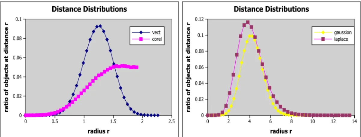
4.1 Distance Distribution for different datasets, including uniform, gaussian and laplace distributions, and color histogram from the corel data. . . 19

4.2 Density around a query object. Green points refer to objects in the sample set. The whole dataset may include other objects within the radius, however the ratio of these objects to the total size is expected to stay the same. . . 21

4.3 The computational overhead for processing objects in the sample set of size = 10000, for different values of k. . . 23

4.4 K-nearest neighbor distances with respect to average pivot dis-tances for objects in the training set of size = 1000. . . 24

LIST OF FIGURES xi

5.1 Relative Errors of global estimations; for ’uniform vector’ and

’corel’ datasets. . . 26

5.2 Proportion of the number of neighbors returned by global

estima-tions; for ’uniform vector’ and ’corel’ datasets. . . 27

5.3 Sample size test for the regression of the query range; for ’uniform

vector’ and ’corel’ datasets. . . 29

5.4 Memory test for the local density method; for ’uniform vector’ and

’corel’ datasets. . . 30

5.5 Relative errors for different k00 values used in the local density

method; k=20,50,100,200; for ’uniform vector’ dataset. . . 32

5.6 Relative errors for different k00 values used in the local density

method; k=20,50,100,200; for ’corel’ dataset. . . 33

5.7 Sample size test for the local density method; k00=20,50,100,200;

for ’uniform vector’ dataset. . . 34

5.8 Sample size test for the local density method; k00=20,50,100,200;

for ’corel’ dataset. . . 35

5.9 Number of pivots test for training method; for ’uniform vector’

and ’corel’ datasets. . . 37

5.10 Relative errors for different methods; for ’uniform’, ’gaussian’,

’laplace’ distributions, ’corel’ data. . . 39

5.11 Number of distance computations for different methods; for

’uni-form’, ’gaussian’, ’laplace’ distributions, ’corel’ data. . . 41

5.12 Ratio of the number of returned neighbors and the size of the back-up list for different methods; for ’uniform’, ’gaussian’, ’laplace’

Chapter 1

Introduction

In computer science, many applications use database management techniques in order to store and retrieve desired data. Complex, unstructured data requires a modeling phase so that it can be represented in some form that can easily be maintained by indexing. For instance, large sized images are generally trans-formed into feature vectors that hold some sort of information about them, such as color, texture, etc... Text documents are also represented as vectors; each di-mension in the vector corresponding to a term in the document. In these vector spaces, the similarity between objects is defined by using geometric distance func-tions like the Euclidean distance. Although a large number of index structures are based on this framework, they lose their effectiveness in higher dimensions. Consequently, a simple, more general framework is developed as an alternative, known as the metric space model.

1.1

Metric Space

A metric space is defined by a set of objects O, and a distance function d between pairs of objects that satisfies the following properties:

CHAPTER 1. INTRODUCTION 2

non-negativity:

∀o1, o2 ∈ O, d(o1, o2) ≥ 0

symmetry:

∀o1, o2 ∈ O, d(o1, o2) = d(o2, o1)

triangle inequality:

∀o1, o2, o3 ∈ O, d(o1, o3) ≤ d(o1, o2) + d(o2, o3) (1.1)

Metric space model provides a high level of abstraction, capturing a high

variety of applications of similarity searching. It does not need to have any

information about the internal structure of the objects, only a distance function that computes the similarity between them is sufficient.

1.2

Similarity Queries

In similarity searching, objects of a set O is classified based on the similarity criteria, which is defined by the distance between the object o and the given query object q.

A range query R(q, r) is defined as:

R(q, r) = o ∈ O : d(q, o) ≤ r

Every object within a distance of r to the query object q is retrieved. The query object itself is not included in the set of objects to be searched. One example of a range query can be: List employees with work experience less than 5 years. A derivation of the range query is defined by not only an upper limit but also a lower limit, where objects with distances in between are retrieved, such as: List employees with 2-5 years of work experience. In Figure 1.1, the objects

CHAPTER 1. INTRODUCTION 3

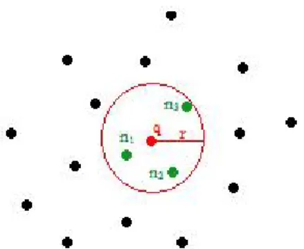
Figure 1.1: Query Radius.

A k-nearest neighbor query kN N (q, k) is defined as:

KNN(q, k) = N ⊂ O, o1 ∈ N, o2 ∈ O-N, |N | = k : d(q, o1) ≤ d(q, o2)

Unlike the range query, the number of neighbors k to be retrieved is specified in the k-nearest neighbor query. The objects are processed in such a way that, a list of neighbors N , of size k, is stored and updated whenever an object closer to the query than the farthest object in N is found, in which case that farthest object is removed. An example for k-nearest neighbor queries can be: List 3

employees having the most least experience. In Figure 1.1, the objects n1, n2, n3

are the 3-nearest neighbors of q. Notice that, the two query examples retrieved the same elements, with different input parameters.

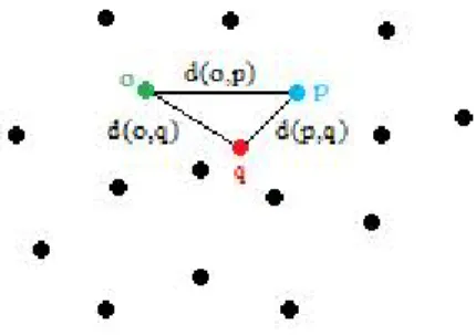
The triangular inequality property of the distance function in Equation 1.1 states that, the distance between two objects is related to their distances to a third object. Using this fact, metric access methods select a group of objects from the database and the rest of the dataset is indexed using these representative or pivot objects.

CHAPTER 1. INTRODUCTION 4

1.3

Indexing Methods

A popular approach used for indexing is to store data objects in a hierarchical way using tree structures. A typical tree node stores a subset of elements cen-tered around a representative object. A covering radius defines the maximum distance of an object from this set to the representative. This information is used for defining distance limits between the query object and the elements in the node. During a range query, elements that stay out of these limits are said to be eliminated from the search space.

Figure 1.2: Limiting Radius and Covering Radius.

Figure 1.3: Distance Bounding.

Another way of indexing is to store objects according to their distances to a group of pre-selected pivot objects. These pre-computed distances are used together with the query object’s distance to the pivot to identify whether a data

CHAPTER 1. INTRODUCTION 5

object is in range of the query object. This technique used for eliminating objects is also referred as pivoting.

Besides tree-structures, there are some other approaches that index data using distance matrices. The pre-computed distances between objects and pivots are stored in array structures and used during query processing. A brief description about index structures recently developed will be presented in the next chapter.

1.4

Radius Estimation

In cases of high dimensional or very complex data, the cost of distance computa-tion is the most important measure for evaluating query performance. For that reason, pruning abilities of metric access methods are very important.

Almost all existing indexing methods perform the technique of eliminating objects using the triangular inequality property of metric spaces, as described in the previous section. Since the maximum distance of an object from the query is known in advance, range queries are performed easily using these pruning abilities. In k-nearest neighbor queries, however, the radius covering the k closest object is not available beforehand. If this distance can be estimated accurately, k-nearest neighbor queries can be reduced to range queries and their performance can improve significantly.

Recently, different approaches are developed for estimating k nearest neighbor distances. Among these are methods that use histograms of distances between objects. In [14], the k nearest neighbors for each pre-selected pivot object are found and their distances are stored in a histogram. These are then used to define an upper bound radius estimate for query object’s k nearest neighbors. Another approach uses a histogram of distances between every pair of objects in a set [21]. A probability density function is then created from this histogram and used for defining the number of object pairs within a given distance. This information is than used to estimate a k-nearest neighbor radius.

CHAPTER 1. INTRODUCTION 6

It has been argued that the distribution of pair-wise distances shows self similarity which means that the properties of the whole dataset is preserved similarly in parts of the dataset. A radius estimation based on this intrinsic dimensionality of datasets is presented in [28].

The performance of a k-nearest neighbor search depends on the overall cost of the query. The number of distance computations required is considered to be the most important evaluator, since it is difficult to calculate the distance between complex data objects. Construction cost, space requirements and CPU overhead are other significant issues that we will mention when comparing different ap-proaches. A detailed explanation of described estimation methods are presented in Chapter 3, together with their overall cost analysis.

In this thesis, we propose several methods for estimating the kthnearest

neigh-bor distance. Our main focus is the precision of estimation and its affect on the performance of the query. We will present detailed comparison of our methods with related approaches in terms of estimation accuracy and disk usage. We will also address the case of underestimation when not enough number of neighbors are returned by the estimated radius. We will show that we outperform other approaches in such cases without the need of another estimation or scan of index data.

The organization of the rest of the thesis is as follows: In Chapter 2, a brief description of common index structures is presented followed by definitions of k-nearest neighbor algorithms based on radius estimation in Chapter 3. Then,

methods for estimating kth _{nearest neighbor distance are proposed in Chapter 4,}

followed by their experimental results in Chapter 5. Finally, in Chapter 6, we present concluding remarks and future work.

Chapter 2

Index Structures

Recent work on similarity searching lead to development of various access meth-ods based on different index structures. Most common approach is to use tree structures for indexing data. Many metric access methods are based on index trees. An alternative solution presented in other methods is to use distance ma-trices for storing distance information among objects.

Indexing methods are evaluated according to their query performance as well as space and construction requirements. Query performance is based on two main measurements: the number of distance calculations, and any additional computation required to process and evaluate these distance measures, referred to as computational overhead. We discuss recent approaches using different index structures.

2.1

Tree-Based Structures

In tree-based index structures the basic theme is to use a hierarchical decompo-sition of the space. One popular approach using tree structures is to partition data into clusters. The objects close to each other are grouped together in these clustering-based methods, where a single object, ideally located near the center of

CHAPTER 2. INDEX STRUCTURES 8

the group is used as the representative. Another approach used in tree structures is to define the partitions based on distance ranges to one or more pivots selected among them. Those with similar distances to these pivot objects are put inside the same subtree; however this does not necessarily indicate that they are also close to each other. The pivots are only used for objects within their subtrees, hence the name local pivots.

The GNAT [1] is an example for tree-based methods, using more than two representatives for a partition. Together with the radius of the region around the representative, the information of the minimum and maximum distances to the objects in every other subset is maintained. Compared to the common local-pivot based structure vp-tree [25], it requires fewer distance computations in exchange of higher construction cost. However, recent experiments [8, 6, 1] show that GNAT performs worse than distance matrix methods in query performance, while it needs less space and computational overhead.

The M-tree [10] and the Slim-tree [22] are disk-based structures which are very similar to the GNAT. In order to support and efficiently process dynamic operations they store less precise data than GNAT, resulting in poorer query performance.

The vp-tree [25] uses a single pivot and a branching factor k to divide objects in a node to k groups differentiated according to their distances to the vantage point. The node itself stores only the k − 1 values defining the distance ranges for each subtree. The shortcoming of the vp-tree is that, for higher dimensions, objects tend to be at similar distances to the pivot, which eliminates the power of distinguishing objects. As an improved version, mvp-tree [2] uses more than one vantage points to further divide the partitions created by other vantage points.

2.2

Distance Matrix Methods

An alternative solution to tree-based structures is to use distance matrices for storing distances between pivots and objects in the dataset. Contrary to local

CHAPTER 2. INDEX STRUCTURES 9

pivot-based methods, each pivot is used in the processing of every object, therefore referred to as global pivots. During query time, these pre-computed distances are used to eliminate objects based on the concept of pivoting. Therefore, a distance computation is required only for those remaining candidate objects which have not been eliminated. With the requirement of higher space and construction time, the global pivot-based methods can boost up query performance by increasing the number of pivots. This is the main advantage of distance matrix methods, since the number of pivots are limited in tree structures decreasing their flexibility to provide enough elimination power especially in high dimensional distributions. In such distributions, there appears a large number objects that are at similar distances to both pivots and the query object. Nevertheless, in global-pivot based methods, as many number of pivots as needed can be used at the expense of higher space and construction cost.

AESA [27] is known to be the first method in which all the data objects also serve as pivots. In LAESA [18], a subset of objects are selected as pivots instead of all of them. The distances between these pivots and rest of the objects are stored in arrays to be used in query time. In the Spaghettis structure [7] , the computational overhead is reduced by sorting these stored distances to pivots and using a binary search among them. This requires, however, additional space and construction time. The Fixed Query Arrays (FQA) [6] eliminates this extra need of space by storing less precise distance values, which reduces the accuracy of pivots especially in high dimensional data.

The main trade-off in distance matrix methods is that, greater query perfor-mance can be achieved in exchange of higher space usage and construction time. A solution for this is proposed in the Kvp structure [5].

2.3

The Kvp Structure

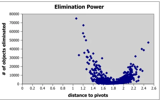
It is shown that a pivot is more effective for objects that are close to or distant from it [5]. This is illustrated in Figure 2.1, where we observe that the number of

CHAPTER 2. INDEX STRUCTURES 10 0 0.2 0.4 0.6 0.8 1 1.2 1.4 1.6 1.8 2 2.2 2.4 2.6 distance to pivots 0 10000 20000 30000 40000 50000 60000 70000 80000 # of objects elimina ted Elimination Power

Figure 2.1: Elimination power with respect to pivot-query distance. objects eliminated by a pivot according to its distance to a query object. In the construction phase, for each object, Kvp stores only the most promising pivot distances based on this information. In order to have effective pivots for every object in the dataset, the selection process is implemented in such a way that objects that are maximally separated from each other are chosen as pivot objects. The selection process is presented in Algorithm 1.

When the next pivot is to be selected, the minimum distances of objects to currently appointed pivots are computed. Then, the object with the maximum value of this distance is chosen as the next pivot. This ensures that selected pivots are distant from the general population, which provides better elimination power.

The prioritization of pivots in Kvp decreases the computational overhead and space requirement, since less number of distances are stored and used. Other than that the same pivoting technique is used similar to other global pivot-based methods.

CHAPTER 2. INDEX STRUCTURES 11

Algorithm 1 Pivot Selection.

Input: set of objects O, number of required pivots nP

Output: the set of pivots P of size nP

define array minDistances of size nO, set all values to inf

select first object o ∈ O as a pivot add o to P

while size of P < nP do

set max to 0

set p to last pivot selected for all o ∈ O − P do

compute d(o,p)

if d(o, p) < minDistance(o) then set minDistance(o) to d(o, p) end if

if max < minDistance(o) then set max to minDistance(o) end if

end for

select o with minDistance(o) = max as the next pivot add o to P

Chapter 3

K-Nearest Neighbor Algorithms

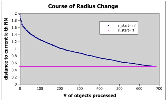
The simplest way of finding k-nearest neighbors of a given query object is to compute its distance to every object in the dataset. This will require n distance computations, where n is the total number of objects. Since this is not accept-able in cases where distance computation is relatively expensive and dominant in overall cost of a query, a lower bounding principle is incorporated in Algorithm 2. 0 100 200 300 400 500 600 700 # of objects processed 0 0.2 0.4 0.6 0.8 1 1.2 1.4 1.6 1.8 2 distance to current k -th NN

Course of Radius Change

r_start=inf r_start=rf

Figure 3.1: The change of the distance to the k-th Nearest Neighbor as more

objects are processed. The straight line shows the value rf.

CHAPTER 3. K-NEAREST NEIGHBOR ALGORITHMS 13

The radius covering the k-nearest neighbors of the query is set to infinity at the beginning. The objects are processed in random order and eliminated accord-ing to their lower bound distances to the query object. Duraccord-ing this operation,

candidate objects are inserted in a list N Nq that contains current nearest

neigh-bors of the query. After N Nq is filled with k neighbors, the radius r is set from

infinity to the distance of the farthest object in the list. The process continues,

updating r whenever a closer object than the current kth _{neighbor in N N}

q is

found.

Algorithm 2 Basic KNN Algorithm. Object-pivot distances are pre-computed. Input: set of objects O, set of pivots P, query q, number of neighbors k

Output: the k -nearest neighbors of q

compute and store distances d(p,q) ∀p ∈ P

set N Nq = list of kNNs of size k

set r = ∞ (distance to kth _NN) for all p ∈ P do if d(p, q) < r then add p to N Nq set r = dmaxN Nq end if end for for all o ∈ O do

compute lower bound value for d(q,o), lb(o) if lb(o) < r then

compute distance d(o,q) if d(o, q) < r then add o to N Nq set r = dmaxN Nq end if end if end for

The shortcoming of this base algorithm is that, since the radius of the k-nearest neighbors starts from infinity, the process can not eliminate a good deal of objects in earlier stages of the process, resulting in high number of distance computations. An example of the change in average r values with respect to number of objects processed, starting from k, is shown in Figure 3.1.

CHAPTER 3. K-NEAREST NEIGHBOR ALGORITHMS 14

The final r value, which we will call rf, is the actual radius of the k-nearest

neighbors of the query object. If this final radius rf had been used to eliminate

objects from the beginning, only objects with lower bounds to the query object

less than rf would have been processed. In other words, for each r value in the

graph, objects with lower bounds between rf and r could be eliminated on top

of the objects that are eliminated by the basic algorithm.

A range query, given the distance to kth _{nearest neighbor as the query radius,}

is therefore the best theoretical algorithm in terms of number of distance com-putations for finding k-nearest neighbors. An equivalent algorithm is presented in K-LAESA [19], which extends LAESA [18] to find k neighbors instead of only 1. The basic approach is to process objects in ascending order of their lower bound of distances to the query object. Candidate objects are added to the cur-rent neighbors list N N q. Whenever an object with a lower bound greater than the farthest object in N N q is found, the algorithm terminates. This way, only the objects with lower bound values smaller than the actual k-nearest neighbor radius are processed, which is exactly the same in the described range query. However, K-LAESA algorithm requires too much construction time and space as well as more than one full scan of index data for the sorting procedure; which also increases the CPU overhead.

A similar approach is also proposed in tree-based structures. An incremental ranking algorithm [13] processes subtrees using a global priority queue, which holds in sorted order the visited nodes and data objects in ascending order of distances, such that the front of the queue holds the element with the smallest distance to the query. The queue is processed in such a way that, if the front of the queue is a node, then its children are added to the priority queue. If it is a data object, it is added as the next nearest neighbor to the N N q. The algorithms stops when N N q is full with required number of neighbors, k. Only the nodes

with distances smaller than the kth _{nearest neighbor distance are traversed. The}

node distances are defined similar to the lower bound distances in distance matrix methods. Therefore, the overall cost is similar to the K-LAESA algorithm.

CHAPTER 3. K-NEAREST NEIGHBOR ALGORITHMS 15

of the kth _{nearest object. As pointed out, a range query would definitely decrease}

the number of distance computations, if the k-nearest neighbor radius could be estimated beforehand. This would also discard the need for a sorting procedure, significantly improving the overall performance of the query processing. For that reason several algorithms estimating the k-nearest neighbor radius are developed. A basic approach is described in [21], where the algorithm uses the information provided by the distance distribution of a dataset. The basic idea is forming histograms of pair-wise distances between objects. Then, this histogram is scaled and viewed as a probability density function as:

H(S) ⇒ P(S, r)

For a dataset of size n, with the requested number of neighbors being k, an

estimate for the distance of the kth nearest neighbor of the query object is then

derived by the following formula.

n

Z E(d(q,KNN(q)))

0

Pq(S, r)dr = k

The probability of finding an object at distance r of the query is computed for a range of values of r, setting the cumulative probability to be k/n. This task requires pre-computed distances among every object, increasing the construction cost significantly.

An extended approach from this method is to take a subset of the described

histogram to form another, storing the distances of objects to their kth nearest

neighbors for all values of k that may be encountered in queries. Using this new histogram a probability density function is created likewise and used for estimating k-nearest neighbor radius for the query object. The following formula

summarizes this approach, where P (k, S, r) is the probability of the kth _neighbor

CHAPTER 3. K-NEAREST NEIGHBOR ALGORITHMS 16

E(d(q, KNN(q))) =

Z ∞

0

rP(k, S, r)dr

Effectively, it is equivalent to taking the average k-th nearest neighbor dis-tances of all the data objects. These two estimation methods are global; meaning that their estimation is same for every possible query object.

Another algorithm that uses histograms is presented in [14]. A small number of pivots are selected from the dataset and their distances to nearest neighbors of them are pre-computed and stored in a matrix. For a given query object,

an upper bound to its kth nearest neighbor is determined using the triangular

inequality property as illustrated in the following formula.

rest = min

1≤i≤m[d(q, pi) + H(pi, KN N (pi))]

The equation implies that, for a certain value of k, the distance between

the query object and a pivot added to the pre-computed kth _{nearest neighbor}

distance of that pivot is definitely larger than the possible distance of the query

to its kth nearest neighbor. Therefore, the minimum upper bound value defined

by m pivots is used as a local estimate. The pivots are selected among the objects minimizing the total value of the pivot distances.

The algorithm requires less space compared to the previous histogram based approaches, storing p.k distances, where p is the number of pivots and k is the number of nearest neighbors. However we will show that it does not estimate an accurate radius which leads to an increased number of distance computations.

The kN N F algorithm in [28] uses the intrinsic dimensionality of datasets for radius estimation. It is described that, the distance distribution between pairs of objects show a fractal behavior, or self similarity. This implies that, certain parts of the dataset shows similar properties to the whole set. Based on this idea, the number of pairs within a certain radius r is defined using the power law.

CHAPTER 3. K-NEAREST NEIGHBOR ALGORITHMS 17

P C(r) = Kp+ rD (3.1)

D is the correlational fractal dimension of the dataset [11], and Kdis a

propor-tionality constant. Based on this relation, the radius of the k-nearest neighbors

is estimated as follows: the logarithm of the constant Kp is derived from (3.1)

using the total number of pairs in the dataset n(n − 1)/2 for P C(r), where n is the database size and R is the maximum distance between two objects.

Kd= log(Kp) = log(n(n − 1)/2) − D log(R) (3.2)

The number of distances between a subset of k objects and the objects of the whole set N is defined as n(k − 1)/2. For a required number of neighbors k, the radius is estimated using the relation in (3.2).

log(n(k − 1)/2) = log(n(n − 1)/2) − D log(R) + D log(rf)

rest = R((log(k−1)−log(n−1))/D)

In case less than required number of neighbors is returned, the same relation is used for a local estimate, only replacing n with the number of retrieved objects

k0 < k, and R with the estimate rest. This way instead of the whole dataset,

only the density around the query object is considered and a more accurate estimation is made. The algorithm uses disk-based index structure slim-tree, as a consequence, this local estimation decreases the performance in terms of disk usage, since it requires another sweep of the index data. However, experiment results show that the local estimation is almost never used, because the global

estimate, rest, is greater than the actual k-nearest neighbor distance most of the

time. This means, the algorithm over estimates the query radius in general, decreasing the number of objects eliminated, therefore increasing the number of distance computations. On the other hand, the algorithm does not require the additional space and construction time for pre-computed distances between objects prior to the query processing.

Chapter 4

Precise Radius Estimation

We have elaborated that a k-nearest neighbor query can be reduced to a range query using a radius estimate. The critical parameter in this transformation is the value of r to be used as an input. We have developed a number of methods for estimating this radius of the k-nearest neighbors of a query, described in the following sections. Their relative errors to the actual distances are discussed in the next chapter, together with the overall performance of the algorithms.

4.1

Global Estimation

A global pair-wise distance distribution is constructed using the pre-computed distances between a sample set of objects from the database. This approach is identical to the one described in [21], except the fact that only a subset of distances is used, decreasing the construction cost. Example distributions for different datasets are shown in Figure 4.1. A certain point on the curve defines the ratio of object pairs at a distance r to the total number of pairs in the dataset. The area under the curve therefore adds up to 1. Observe that the percentage of objects that are close to or distant from each other is relatively small compared to the rest of the dataset.

CHAPTER 4. PRECISE RADIUS ESTIMATION 19 0 0.5 1 1.5 2 2.5 radius r 0 0.02 0.04 0.06 0.08 0.1 ratio of objects at di stance r Distance Distributions vect corel 0 2 4 6 8 10 12 14 radius r 0 0.02 0.04 0.06 0.08 0.1 0.12 ratio of objects at di stance r Distance Distributions gaussion laplace

Figure 4.1: Distance Distribution for different datasets, including uniform, gaus-sian and laplace distributions, and color histogram from the corel data.

A global estimation is made using the distance distribution. A cumulative probability function is defined using the area under the curve for a range of r values.

F (r) = number of distances ≤ r

total number of distances

The F (r) function is used to find the number of objects in range r of a given query object q, the number of distances less than r between q and any data object o. The ratio that F (r) returns is multiplied by the total number of objects at any distance to q, which is the size of the database n.

Consequently, the reverse of the function F (r) estimates a radius for a given number of required neighbors k.

F−1(k

N) = r (4.1)

A significant problem with global estimation is that it gives the same radius for any possible query object. Therefore by definition, although accurate on average, it will give an overestimate for half of the query objects, and an underestimate for the other half. The former will increase the number of distance computations, whereas in the latter case, not enough neighbors would be returned. For that

CHAPTER 4. PRECISE RADIUS ESTIMATION 20

reason, an estimation considering the query location is crucial in precision of the radius estimate. Even though global estimation is not adequate by itself, it is incorporated in some local estimation methods described in the following sections.

4.2

Local Estimation

A query object, due to its distinct location, may not abide by the general distri-bution of pair-wise distances. In that case, the location of the query object needs to be considered. One approach is to select a sample of objects from the dataset to be processed for a local estimation. Since this sample set is stored in the memory, this procedure is done efficiently, without the requirement of additional disk scans.

4.2.1

Progress Of Query Range

Regression is a technique used to model a numerical data consisting of values of a dependent variable, and one or more independent variables. It is commonly used for prediction. There are several types of regression for fitting (least squares fitting) a curve through a given set of points. The change of the dependent

variable; distance of the current kth _{nearest neighbor, along with the number of}

objects processed follows that of a power law distribution illustrated in Figure 3.1 on Page 12 defined by the function:

y = a · xb

The sample objects in memory are processed using the base algorithm on Page 13. The change of the radius value together with the number of objects processed is given as input to the regression function. Then, given the total number of objects in the dataset, the final radius is predicted, which is used as a local estimation of the query object.

CHAPTER 4. PRECISE RADIUS ESTIMATION 21

A shortcoming of this method is that the objects processed in memory need to be reconsidered after the radius estimation. The reason is that they may or may

not lay in the range rest of the query. This is overcome by using an array storing

the already computed distances of objects in the sample set. This eliminates the need of redundant distance re-computation for these objects.

4.2.2

Uniformity of Local Density

Due to the self similarity of the dataset, regardless of the total number of objects, the density around the query stays at similar levels. This suggests that if the

distance of the kth nearest neighbor among a subset of objects of size m is r for

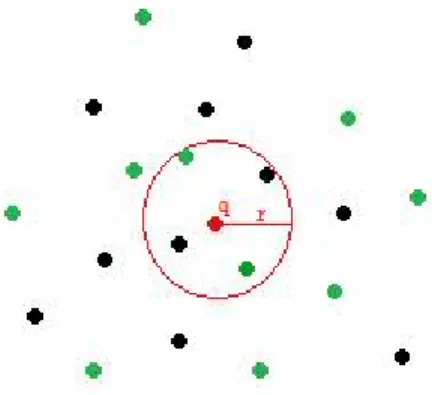
a given query, then the radius for k ∗ n/m nearest neighbors in the whole set will also be r. This is illustrated in Figure 4.2, where green points are sampled objects of size m=10, where n=20. Based on this observation, the sample objects

in memory are processed using the base algorithm, finding the k0 = k ∗ m/n

nearest neighbors. The distance of the farthest object in this list is then used as a local estimation.

Figure 4.2: Density around a query object. Green points refer to objects in the sample set. The whole dataset may include other objects within the radius, however the ratio of these objects to the total size is expected to stay the same.

CHAPTER 4. PRECISE RADIUS ESTIMATION 22

An important parameter for this method is, like in the previous method, the number of objects to be sampled and processed in memory. There are some serious restrictions on the sample size. For instance, if k is a small value such as

5, the sample must be at least one fifth of the whole dataset so that k0 can be set

to at least 1. This shortcoming is addressed in a modified version of this method, in cases when significant increase to the memory size is unavailable.

Projection of Distance Distribution

If the k value is very small, then it becomes impractical to have a meaningful

value for k0 while keeping the sample size small. For such cases, we propose a

new method based on the observation that while the distance of the kth _neighbor

is expected to be different for different query objects, it will be proportional for different values of the number of neighbors. For example, if the distance of the

5th nearest neighbor is above average by 20%, then we also expect the distance

of the 10th _{nearest neighbor to be about 20% higher than the average. Based on}

this, whenever k0 is too small, we will use another value k00 that will let us use

less samples.

Recall the reverse cumulative probability function in Equation 4.1 on Page

19. The previous method states that for k0 = k ∗ m/n,

F−1(k 0 m) = F −1 (k n)

Another parameter, k00, is introduced in this method indicating the minimum

number of neighbors to be retrieved among the sample objects in memory, whose radius will be used for estimation.

r(k0) r(k00₎ = F−1(k_n) F−1₍k00 m) (4.2)

The left side in the Equation 4.2 illustrates the radius of the neighbors, k0 and

k00 > k0 respectively, among sample objects in memory. Since k0 and therefore

CHAPTER 4. PRECISE RADIUS ESTIMATION 23

estimations for both values, the radius of k nearest neighbors of the query in the

whole set is estimated. Recall from previous method that r(k0) in m objects is

expected to be similar to r(k) in n objects.

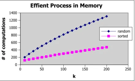
The processing of the sample set of data objects increases the computational overhead, though it does not affect number of distance computations, since they are stored and reused during query processing with the estimated radius. Fur-thermore, considering they are processed in memory, efficiency can be improved by using the lower bound sorting algorithm described in [19]. The result of this modification is shown in Figure 4.3.

0 50 100 150 200 250 k 0 200 400 600 800 1000 1200 1400 # of computations

Effient Process in Memory

random sorted

Figure 4.3: The computational overhead for processing objects in the sample set of size = 10000, for different values of k.

We will emphasize the effect of the sample objects size and the k00 value in

the experimental results.

4.2.3

Static Pivots

As mentioned before, the location of the query object affects the expected radius of its k nearest neighbors. A second approach to identify the query whereabouts is by use of pivot distances. For instance, if an object is far away from the general population its neighbors will also be relatively farther than expected. Similarly, if it’s too close to the set of objects, its radius will be smaller than expected.

CHAPTER 4. PRECISE RADIUS ESTIMATION 24

In order to isolate the location of the query, its distance to a set of appointed pivot objects are computed. We expect those with a large value of average dis-tance to pivots to have larger radius for its k nearest neighbors, and vice verse.

A learning phase is carried out based on the relationship between an object’s distance to its pivots and k nearest neighbors. A sample set of objects are

se-lected for training and processed observing the values, dknn(q) and davg(q, p). A

regression technique similar to the one described before is used for modeling the relation between these distance values. We observe from Figure 4.4 that there is almost a linear dependency in the relation.

1.2 1.3 1.4 1.5 1.6 1.7 1.8

average distance to pivots

0 0.1 0.2 0.3 0.4 0.5 0.6 0.7 0.8 distance to k-th nea rest neighbor

Relation of Distances to Pivots and Neighbors

k=50 k=100 k=200

Figure 4.4: K-nearest neighbor distances with respect to average pivot distances for objects in the training set of size = 1000.

Prior to processing the objects in the dataset for determining the k nearest neighbors of a query, its pivot distances are computed. The average is then used

for predicting the distance of the kth_{nearest neighbor from the regression model,}

which is then used as a local estimation. We will illustrate the effect of the number of pivots appointed for use in the estimation.

Chapter 5

Experiment Results

Throughout the experiments, we have used several datasets, including uniform and non-uniform distributions. Along with the random vector sets with uniform, laplace and gaussian distributions of size 100k and dimension 10, we processed the color histogram of size 68040 and dimension 32 from the Corel data.

We have tested 100 samples of query objects for each dataset. Since average error values of the radius may not show the actual accuracy of the estimation, we used the term relative error in order to describe the effectiveness of the algorithms. Along with relative error, we present the number of distance computations, and the number of neighbors retrieved by the estimated radius to illustrate how much of the backup list of objects need to be processed to reach the requested number of neighbors k.

5.1

Global Estimations

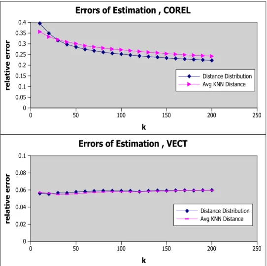
Including the algorithms presented in [21], we tested the global estimation derived from the sample distance distribution. Recall that the first approach in [21] and our global estimation are similar except only use different sizes of samples. The errors of estimations are illustrated for different datasets in Figure 5.1.

CHAPTER 5. EXPERIMENT RESULTS 26 0 50 100 150 200 250 k 0 0.05 0.1 0.15 0.2 0.25 0.3 0.35 0.4 relative error

Errors of Estimation , COREL

Distance Distribution Avg KNN Distance 0 50 100 150 200 250 k 0 0.02 0.04 0.06 0.08 0.1 relative error

Errors of Estimation , VECT

Distance Distribution Avg KNN Distance

Figure 5.1: Relative Errors of global estimations; for ’uniform vector’ and ’corel’ datasets.

CHAPTER 5. EXPERIMENT RESULTS 27

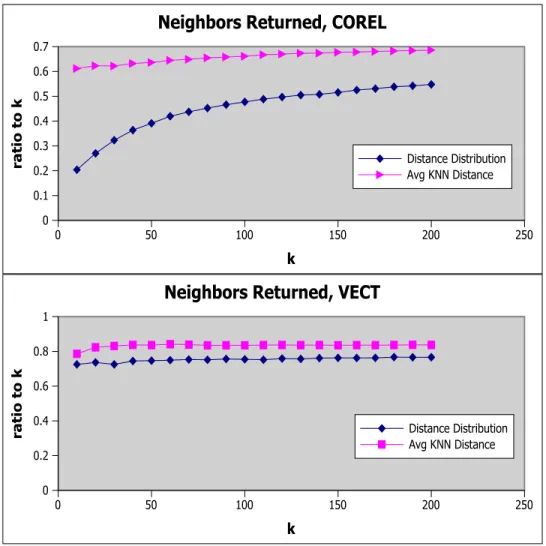
The key observation from the resulting graphs is that, especially for uniform data, a global estimate is very close to the actual radius of the neighbors in average. However, this does not necessarily mean that it is accurate for each specific query. Quite the contrary, the method overestimates for one half of the queries, and underestimate for the other half, returning less than required number of neighbors. The ratio of the number of neighbors returned to k is illustrated in Figure 5.2. 0 50 100 150 200 250 k 0 0.1 0.2 0.3 0.4 0.5 0.6 0.7 ratio to k

Neighbors Returned, COREL

Distance Distribution Avg KNN Distance 0 50 100 150 200 250 k 0 0.2 0.4 0.6 0.8 1 ratio to k

Neighbors Returned, VECT

Distance Distribution Avg KNN Distance

Figure 5.2: Proportion of the number of neighbors returned by global estimations; for ’uniform vector’ and ’corel’ datasets.

CHAPTER 5. EXPERIMENT RESULTS 28

5.2

Local Estimations

As we described in the previous chapter, several techniques for identifying the location of the query is used in order to perform a local estimation. In exchange of increasing the computational overhead, all approaches give more accurate results compared to global estimation.

5.2.1

Progress of Query Range

A common approach used for prediction over a distribution of points is to use the regression model. An important parameter for this method is the number of independent variables used for the input data. This corresponds to the size of the sample set processed for estimation. The significance of this size is observed in Figure 5.3.

We see that in corel data, the effect of increasing the sample size descents at a slow rate. In uniform vectors however, larger sample size becomes irrelevant after a certain value, especially for bigger values of k. Since increasing sample size signifies additional computation, limiting it to a reasonable value is essential. Based on these observations, we define the sample set size to be a tenth of the total data size. Smaller values also perform well, especially in uniform data, however, we selected this value for fair comparison with other methods.

5.2.2

Uniformity of Local Density

The second idea is to process a sample set of objects and draw a conclusion about the density around the query. Recall that for a certain radius, although the number of neighbors of an object changes by increasing the total data size, its ratio to the whole set stays the same. Again, the size of the sample set is a key parameter. In Figure 5.4, the effect of the number of objects processed is represented in terms of relative error.

CHAPTER 5. EXPERIMENT RESULTS 29 0 5000 10000 15000 20000 25000 Sample Size 0 0.02 0.04 0.06 0.08 0.1 0.12 0.14 Relative Error

Sample Size Test - Regression

k=10 k=50 k=100 k=150 k=200 0 2000 4000 6000 8000 10000 12000 14000 16000 18000 Sample Size 0 0.1 0.2 0.3 0.4 0.5 Relative Error

Sample Size Test - Regression

k=50 k=100 k=150 k=200

Figure 5.3: Sample size test for the regression of the query range; for ’uniform vector’ and ’corel’ datasets.

CHAPTER 5. EXPERIMENT RESULTS 30 0 5000 10000 15000 20000 25000 Sample Size 0 0.02 0.04 0.06 0.08 0.1 0.12 0.14 Relative Error

Sample Size Test - Local Density

k=10 k=20 k=50 k=100 k=200 0 2000 4000 6000 8000 10000 12000 14000 16000 18000 Sample Size 0 0.02 0.04 0.06 0.08 0.1 0.12 0.14 Relative Error

Sample Size Test - Local Density

k=10 k=20 k=50 k=100 k=200

Figure 5.4: Memory test for the local density method; for ’uniform vector’ and ’corel’ datasets.

CHAPTER 5. EXPERIMENT RESULTS 31

It can be observed that for small sizes of the sample set, the error increases.

The reason is, the number of neighbors k0to be found becomes too low, decreasing

the quality of the estimation. This can be related to the observation described earlier that the general distribution fails to successfully express the distance ratio for close objects. Also a conclusion can be made for the optimal size of the sample set, as its effect does not improve much after a certain value.

Projection of Distance Distribution

The shortcoming of this method comes through for small values of k0, which is

the number of neighbors to be retrieved for estimation. In cases where the size of

the sample set can not be increased much, a new parameter k00 is used to replace

k0 when it’s too small. Experiments for identifying an optimum value for k00 are

presented in Figures 5.5-5.6 for different values of k.

An important observation from these results is that, greater values of k00

ac-tually decreases the precision for corel data. The reason behind this is the global

estimation used in proportioning in Equation 4.2 on Page 22. High values of k00

increases the affect of this ratio on the estimated k0 radius, which also defines the

actual k nearest neighbor distance. For uniform data the opposite is the case,

where increasing k00 also increases the accuracy of the estimation, however in a

slow rate for very high values.

The important point to be discussed in these experiments is that, increasing the sample set size also increases the computational overhead. The lower bound sorting approach is also applicable in this method since the only difference is to

use k00> k0 instead of small k0 values. The required computations in memory for

estimation is shown in Figures 5.7-5.8.

We decided to use 0.1 sampling rate for these methods, since for lower values,

k0 becomes less than 1 in which case the local density algorithm malfunctions.

Using smaller sizes does not increase the error much, however, using the lower bound sorting technique, computational overhead can be minimized, and there-fore higher number of sample objects can be efficiently processed.

CHAPTER 5. EXPERIMENT RESULTS 32 0 2000 4000 6000 8000 10000 12000 14000 16000 18000 20000 22000 Sample Size 0 0.005 0.01 0.015 0.02 0.025 0.03 0.035 0.04 0.045 0.05 0.055 Relative Error k'' test for k=20 k''=5 k''=10 k''=20 k''=40 k''=80 0 5000 10000 15000 20000 25000 Sample Size 0 0.01 0.02 0.03 0.04 0.05 0.06 Relative Error k'' test for k=50 k''=5 k''=10 k''=20 k''=40 k''=80 0 5000 10000 15000 20000 25000 Sample Size 0 0.01 0.02 0.03 0.04 0.05 Relative Error k'' test for k=100 k''=5 k''=10 k''=20 k''=40 k''=80 0 5000 10000 15000 20000 25000 Sample Size 0 0.01 0.02 0.03 0.04 0.05 Relative Error k'' test for k=200 k''=5 k''=10 k''=20 k''=40 k''=80

Figure 5.5: Relative errors for different k00values used in the local density method;

CHAPTER 5. EXPERIMENT RESULTS 33 0 2000 4000 6000 8000 10000 12000 14000 Sample Size 0 0.1 0.2 0.3 0.4 Relative Error k'' test - k=20 k''=5 k''=10 k''=20 k''=40 k''=80 0 2000 4000 6000 8000 10000 12000 14000 16000 18000 Sample Size 0 0.1 0.2 0.3 0.4 Relative Error k'' test for k=50 k''=5 k''=10 k''=20 k''=40 k''=80 0 2000 4000 6000 8000 10000 12000 14000 16000 18000 Sample Size 0 0.05 0.1 0.15 0.2 0.25 0.3 0.35 Relative Error k'' test for k=100 k''=5 k''=10 k''=20 k''=40 k''=80 0 2000 4000 6000 8000 10000 12000 14000 16000 18000 Sample Size 0 0.05 0.1 0.15 0.2 0.25 0.3 Relative Error k'' test for k=200 k''=5 k''=10 k''=20 k''=40 k''=80

Figure 5.6: Relative errors for different k00values used in the local density method;

CHAPTER 5. EXPERIMENT RESULTS 34 0 2000 4000 6000 8000 10000 12000 14000 16000 18000 20000 22000 sample size 0 1000 2000 3000 4000 5000 # of computations

Computational Overhead , k=20 , VECT

k''=5 k''=10 k''=20 k''=40 k''=80 0 5000 10000 15000 20000 25000 sample size 0 1000 2000 3000 4000 5000 # of computations

Computational Overhead , k=50 , VECT

k''=5 k''=10 k''=20 k''=40 k''=80 0 5000 10000 15000 20000 25000 sample size 0 1000 2000 3000 4000 5000 # of computations

Computational Overhead , k=100 , VECT

k''=5 k''=10 k''=20 k''=40 k''=80 0 5000 10000 15000 20000 25000 sample size 0 1000 2000 3000 4000 5000 # of computations

Computational Overhead , k=200 , VECT

k''=5 k''=10 k''=20 k''=40 k''=80

Figure 5.7: Sample size test for the local density method; k00=20,50,100,200; for

CHAPTER 5. EXPERIMENT RESULTS 35 0 2000 4000 6000 8000 10000 12000 14000 sample size 0 500 1000 1500 2000 2500 3000 # of computations

Computational Overhead , k=20, COREL

k''=5 k''=10 k''=20 k''=40 k''=80 0 2000 4000 6000 8000 10000 12000 14000 16000 18000 sample size 0 500 1000 1500 2000 2500 3000 # of computations

Computational Overhead , k=50 , COREL

k''=5 k''=10 k''=20 k''=40 k''=80 0 2000 4000 6000 8000 10000 12000 14000 16000 18000 sample size 0 500 1000 1500 2000 2500 3000 # of computations

Computational Overhead , k=100 , COREL

k''=5 k''=10 k''=20 k''=40 k''=80 0 2000 4000 6000 8000 10000 12000 14000 16000 18000 sample size 0 500 1000 1500 2000 2500 3000 # of computations

Computational Overhead , k=200 , COREL

k''=5 k''=10 k''=20 k''=40 k''=80

Figure 5.8: Sample size test for the local density method; k00=20,50,100,200; for

CHAPTER 5. EXPERIMENT RESULTS 36

The value of k00 is decided as 20, because larger values decrease performance

for real datasets and only increase accuracy slightly for uniform data.

A key note is that for especially different sizes and dimensions these values can be altered for optimizing performances. Our choices are merely for fair com-parison between different approaches.

5.2.3

Static Pivots

Another approach to estimate the location of the query is by use of pivots. As mentioned before, a query is assumed distant to general population if its average distance to pivots is greater than expected. The effectiveness of the method based on the size of the pivot objects set is illustrated in Figure 5.9.

We see that the effect of changing the number of pivots differs according to the type of data. The increase in the number of pivots improves for corel data. However, we observe that after a certain value it has negative effect on accuracy of the estimation. This value changed for different experiments. In Figure 5.9, we see 500 pivots perform worse than using 300 pivots. On uniform data, on the other hand, the precision does not change considerably. This may be related to the low dimension size, since the precision is already very good.

Another important matter here is an increase in pivots size means higher com-putation during both construction time and radius estimation. For that reason, the positive effect of high number of pivots is insignificantly low compared to these costs, therefore 100 pivots were used during experiments. However, a bet-ter estimation can be made using 300 pivots, which may have significant effect on larger data sizes and dimensions, in exchange of a small increase in computational cost.

We will show the local estimations clearly perform better than global versions. The effect of the consideration of the query location is the main reason behind this. In methods that use the uniformity of local density, the CPU overhead is minimized by processing sample objects in sorted order of their lower bounds.

CHAPTER 5. EXPERIMENT RESULTS 37 0 50 100 150 200 250 k 0 0.005 0.01 0.015 0.02 0.025 0.03 0.035 relative error

# Of Pivots Regression Test , VECT

p=100 p=200 p=300 p=400 p=500 0 50 100 150 200 250 k 0.29 0.3 0.31 0.32 0.33 0.34 0.35 0.36 0.37 relative error

# Of Pivots Regression Test , COREL

p=100 p=200 p=300 p=400 p=500

Figure 5.9: Number of pivots test for training method; for ’uniform vector’ and ’corel’ datasets.

CHAPTER 5. EXPERIMENT RESULTS 38

However, the basic algorithm is used for regression of the query range, since the course of r is analyzed. This results in poorer performance in terms of number of computations. The training phase for static pivots does not require much additional computation, since pivot distances of every object are already pre-computed.

5.3

Overall Comparison

As we clarified, the performance of radius estimation can best be represented

by its relative error over the actual kth _{nearest neighbor distance. Besides that,}

the number of distance computations is compared along with the number of

neighbors retrieved. An important relation between these two is that, when

not enough neighbors are found, each algorithm continues to find the remaining neighbors using the lower bound sorting solution. This results in lower number of computations which may distort the performance measure by itself.

Lines in the graphics represents methods as follows:

GLOBAL Global estimation using distance distribution

AVG-KNND Global estimation using the average kth_{nearest neighbor distance}

LOCALD Estimation considering the local density around the query DDPROP Same as LOCALD, except k” parameter is used for low k’ values

REG Estimation from regression of <r distance> for objects processed in memory FD Estimation using the fractal dimensionality of the data

HIST1 Estimation using histogram of pivots kth_{nearest neighbor distances}

P-REG Estimation from regression of <average pivot distance, kth_{nearest neighbor distance>}

The local estimation methods give better results compared to the global es-timation approaches. In Figure 5.10, we see that the static pivots method using the information of average distances to pivots gives the best precision for esti-mation in uniform data. In difficult distributions, however, such as corel data, performance of methods using the information of local density gives better

re-sults relative to static pivots method. Local density method using k00 parameter

CHAPTER 5. EXPERIMENT RESULTS 39 0 50 100 150 200 250 k 0 0.02 0.04 0.06 0.08 0.1 relative error

Relative Errors , VECT _{P_REG}

AVG_KNND DDPROP GLOBAL LOCALD REG 0 50 100 150 200 250 k 0 0.2 0.4 0.6 0.8 1 1.2 1.4 1.6 1.8 2 2.2 relative error

Compared Algorithms , VECT

FD HIST1 0 50 100 150 200 250 k 0 0.02 0.04 0.06 0.08 0.1 0.12 0.14 0.16 0.18 relative error

Relative Errors , GAUSSIAN

P_REG AVG_KNND DDPROP GLOBAL LOCALD REG 0 50 100 150 200 250 k 0 0.2 0.4 0.6 0.8 1 1.2 1.4 1.6 1.8 2 2.2 relative error

Compared Algorithms , GAUSSIAN

FD HIST1 0 50 100 150 200 250 k 0 0.05 0.1 0.15 0.2 0.25 relative error

Relative Errors , LAPLACE

P_REG AVG_KNND DDPROP GLOBAL LOCALD REG 0 50 100 150 200 250 k 0 0.5 1 1.5 2 2.5 3 3.5 relative error

Compared Algorithms , LAPLACE

FD HIST1 0 50 100 150 200 250 k 0 0.1 0.2 0.3 0.4 relative error

Relative Errors , COREL

P_REG AVG_KNND DDPROP GLOBAL LOCALD REG 0 50 100 150 200 250 k 0 0.5 1 1.5 2 2.5 3 relative error

Compared Algorithms , COREL

FD HIST1

Figure 5.10: Relative errors for different methods; for ’uniform’, ’gaussian’, ’laplace’ distributions, ’corel’ data.

CHAPTER 5. EXPERIMENT RESULTS 40

both cases the performance of algorithms using histograms and the fractal di-mension fails to estimate the radius accurately. The increase in the relative error results from overestimation as the algorithms give significantly larger radius

val-ues compared to the actual kth _{nearest neighbor distance. Although they return}

all k nearest neighbors, the number of distance computations rise excessively. A comparison of the estimation methods in terms of distance calculations is shown in Figure 5.11.

The methods using regression for the progress of the query range performs poorly, because of the inefficient processing of objects in the sample set. The reason is, as described, the objects are processed randomly, instead of in sorted order, so as to predict the course of the r value.

We observe that in terms of distance calculations, global estimations give similar results to local methods. This is actually insignificant, because the global estimation methods retrieve less number of neighbors, therefore requiring larger sizes of backup list. Since the candidate objects in this list is processed using the lower bound sorting approach, the total number of distance computations is kept in minimal values. The Figure 5.12 illustrates these observations.

We see that the less number of neighbors retrieved, the more objects the algorithm requires in the backup list. For some queries, global estimation retrieve even 0 neighbors therefore all the k-nearest neighbor are found from the backup list. In cases of higher dimensions and larger database sizes, this is unacceptable since the approach sorts the objects requiring additional disk scan and high CPU usage.

CHAPTER 5. EXPERIMENT RESULTS 41 0 50 100 150 200 250 k 0 2000 4000 6000 8000 10000 12000 # of distance compu tations

Distance Computations, VECT

HIST1 FD REG AVG_KNND GLOBAL LOCALD DDPROP P_REG KLAESA

HIST1 FD REG AvgD GLB LD DDP Preg KLAESA

0 2000 4000 6000 8000 10000 12000 DC , k=200 0 50 100 150 200 250 k 0 2000 4000 6000 8000 10000 12000 # of distance compu tations

Distance Computations, GAUSSIAN

HIST1 FD REG AVG_KNND GLOBAL LOCALD DDPROP P_REG KLAESA

HIST1 FD REG AvgD GLB Preg LD DDP KLAESA

0 1000 2000 3000 4000 5000 6000 7000 8000 9000 10000 11000 DC , k=200 0 50 100 150 200 250 k 0 2000 4000 6000 8000 10000 # of distance compu tations

Distance Computations , LAPLACE

HIST1 FD REG AVG_KNND GLOBAL LOCALD DDPROP P_REG KLAESA

HIST1 FD REG AvgD GLB Preg LD DDP KLAESA

0 1000 2000 3000 4000 5000 6000 7000 8000 9000 DC , k=200 0 50 100 150 200 250 k 0 2000 4000 6000 8000 10000 # of distance compu tations

Distance Computations , COREL

HIST1 FD REG AVG_KNND GLOBAL LOCALD DDPROP P_REG KLAESA

HIST1 FD REG Preg AvgD GLB LD DDP KLAESA

0 1000 2000 3000 4000 5000 6000 7000 8000 9000 DC , k=200

Figure 5.11: Number of distance computations for different methods; for ’uni-form’, ’gaussian’, ’laplace’ distributions, ’corel’ data.

CHAPTER 5. EXPERIMENT RESULTS 42 0 50 100 150 200 250 k 0.4 0.5 0.6 0.7 0.8 0.9 1 1.1 neighbors found / k NNs Returned , VECT P_REG AVG_KNND DDPROP FD HIST1 GLOBAL LOCALD REG 0 50 100 150 200 250 k 0 200 400 600 800 1000 # of computations

Backup List Usage , VECT

P_REG AVG_KNND DDPROP FD HIST1 GLOBAL LOCALD REG 0 50 100 150 200 250 k 0 0.1 0.2 0.3 0.4 0.5 0.6 0.7 0.8 0.9 1 1.1 neighbors found / k NNs Returned , GAUSSIAN P_REG AVG_KNND DDPROP FD HIST1 GLOBAL LOCALD REG 0 50 100 150 200 250 k 0 500 1000 1500 2000 # of computations

Backup List Usage , GAUSSIAN

P_REG AVG_KNND DDPROP FD HIST1 GLOBAL LOCALD REG 0 50 100 150 200 k 0 0.1 0.2 0.3 0.4 0.5 0.6 0.7 0.8 0.9 1 1.1 neighbors found / k NNs Returned , LAPLACE P_REG AVG_KNND DDPROP FD HIST1 GLOBAL LOCALD REG 0 50 100 150 200 k 0 500 1000 1500 2000 # of computations

Backup List Usage , LAPLACE

P_REG AVG_KNND DDPROP FD HIST1 GLOBAL LOCALD REG 0 50 100 150 200 250 k 0 0.2 0.4 0.6 0.8 1 1.2 neighbors found / k NNs Returned , COREL P_REG AVG_KNND DDPROP FD HIST1 GLOBAL LOCALD REG 0 50 100 150 200 250 k 0 500 1000 1500 2000 2500 3000 # of computations

Backup List Usage , COREL

P_REG AVG_KNND DDPROP FD HIST1 GLOBAL LOCALD REG

Figure 5.12: Ratio of the number of returned neighbors and the size of the back-up list for different methods; for ’uniform’, ’gaussian’, ’laplace’ distributions, ’corel’ data.

Chapter 6

Conclusion

In this thesis, we have presented an efficient k-nearest neighbor algorithm based on precise radius estimation. We proposed query processing using only one sequential scan of the index data, even not enough number of neighbors are retrieved by the estimation. A list storing the promising candidates for the remaining neighbors is shown to be kept at reasonable sizes by the accurate estimation of the k-nearest neighbor radius.

We have demonstrated the performance of different estimation methods em-phasizing the amount of space and computation requirements. We illustrated their precision in terms of relative errors and the number of neighbors returned. We have shown that we outperform related algorithms using radius estimation without the requirement of significant computational overhead.

For uniform data, average pivot distances give precise information about the neighborhood of the query object, giving the best results compared to each other algorithm. On the other hand, the local density methods are shown to perform better compared to the static pivots method on difficult distributions. The reason behind this is, for non-uniform datasets, the distribution of pivots over the general population does not give precise information about the location of the query object. Since the density around a specific query is considered each time, other local estimation methods are not affected by difficult distributions that much.

CHAPTER 6. CONCLUSION 44

6.1

Future Work

A number of improvements can be made to the proposed algorithm, especially regarding the local estimation methods. We have observed that the effect of the sample size changes for different values of k. Furthermore, it varies for different processing of the set. For regression of the query range method, for instance, the sampling rate can be decreased without losing much performance. This could de-crease the computational overhead. The number of objects in the sample set can

also be adjusted better for local density method when k00 is used as a parameter,

since they have similar effects on the quality of the estimation.

Clustered data sets have different characteristics and we have tried different versions of the static pivots method. Instead of average values to all pivots, a single close pivot object can be considered, in order to obtain precise information about the cluster that the neighbors of the query object lies within. Similar ideas can also be adjusted for other local estimation methods.

Bibliography

[1] Sergey Brin. Near neighbor search in large metric spaces. In The VLDB Journal, pages 574584, 1995.

[2] Tolga Bozkaya and Meral Ozsoyoglu. Distance-based indexing for high-dimensional metric spaces. In SIGMOD 97: Proceedings of the 1997 ACM SIGMOD international conference on Management of data, pages 357368, New York, NY, USA, 1997. ACM Press.

[3] C. Celik. Priority vantage points structures for similarity queries in metric spaces. In Proceedings of EurAsia-ICT, volume 2510 of Lecture Notes in Computer Science, pages

[4] C. Celik. Effective use of space for pivot-based metric indexing structures. In: Proc.of Int. Workshop on Similarity Search and Applications (SISAP 2008), Cancn,Mxico, IEEE

[5] C. Celik New Approaches to Similarity Searching in Metric Spaces. PhD. Thesis.

[6] Edgar Chavez, Jose L. Marroqun, and Gonzalo Navarro. Fixed queries array: A fast and economical data structure for proximity searching. Multimedia Tools Appl., 14(2):113135, 2001.

[7] Edgar Chavez, Jose L. Marroqun, and Ricardo A. Baeza-Yates. Spaghet-tis: An array based algorithm for similarity queries in metric spaces. In SPIRE/CRIWG, pages 3846, 1999.